Full Handbook: Difference between revisions
(Created page with "This page lets you read the wiki content in a more traditional '''handbook''' format, with all wiki pages combined into a single page for easier reading. See Handbook for...") |
mNo edit summary |
||
| Line 5: | Line 5: | ||
<!-- | <!-- | ||
Note to editors: | Note to editors: | ||
| Line 15: | Line 14: | ||
Once you have saved your edit, | Once you have saved your edit, | ||
the changes will also appear in the handbook. | the changes will also appear in the handbook. | ||
--> | --> | ||
__TOC__ | __TOC__ | ||
Latest revision as of 12:29, 17 November 2022
This page lets you read the wiki content in a more traditional handbook format, with all wiki pages combined into a single page for easier reading.
See Handbook for a split version with one page per chapter.
General
Installation
Which version should I use?
See our homepage for an overview of the available versions of ProB. All ProB tools can be downloaded from our Download page.
The standalone version Tcl/Tk of ProB contains a richer set of features than the Rodin version and also works on other formalisms than Event-B (e.g., classical B, Z, CSP, B||CSP, Promela, ...). If you want to do animation and model checking of Event-B models, the Rodin version might be enough. The Rodin version contains a translation tool from Rodin into Event-B package files that can be used within the standalone version of ProB. Use the probcli version if you want to write batch scripts or prefer working from the command-line.
Installation Instruction for ProB (Standalone)
Note: we have specific Windows_Installation_Instructions. These here are the generic instructions.
- Obtain your platform specific ProB distribution from Downloads. Decompress and expand the ProB directory if necessary. Do not change the location and structure of the files and directories within ProB (apart from the Machines directory)! On Windows you just have to double-click the installer. The contents of the ProB directory should look something like this:
examples            lib     prob
StartProB.sh        tcl
On Windows, you will also have a subfolder called "Microsoft.VC80.CRT" containing the DLLs for the C runtime. Also, the binary is called "ProBWin" and not "prob".
- Be sure that you have Tcl/Tk installed (see, e.g., http://www.tcl.tk/software/tcltk/).
With the latest version of ProB, you have to install Tcl/Tk version 8.5. For example, you can find a correct version of Tcl/Tk athttp://downloads.activestate.com/ActiveTcl/releases/8.5.18.0/ .
- To load your own B machines you also need Java 7 or newer runtime or better JDK.
- Note: you can skip this step if you do not wish to use the visualization commands. Install the "dot" program and "dotty" viewer from AT&T's Graphviz package (http://www.graphviz.org/ or http://www.research.att.com/sw/tools/graphviz/). By default, ProB will open the "dotty" program to visualize the graphs, but postscript viewers (such as gv) are also supported. So, you do not need to install dotty if you don't want to; but it is probably easiest to install the entire Graphviz package.
- Change to the ProB directory and then start up prob. In Windows you can simply double-click on the ProBWin Application. On Mac OS X you may have to type 'limit data unlimited' (in tcsh) or 'ulimit -d unlimited' (in bash) before launching ProB using the Terminal Application. The distribution contains a script StartProB.sh which does this for you (note you may have to do chmod u+x StartProB.sh before launching it from the command-line).
- Now you should be able to open some of the B Machines in the Machines directory. You should then be able to initialize the machines and animate them. Have a look at the supplied Machines in the examples directory. Have fun ! Please report bugs!
Checklist/Troubleshooting
- Java: be sure to have Java 7 or newer installed. Otherwise you will not be able to parse your own classical B machines as our parser is written in Java.
- Tcl/Tk: be sure to have a suitable version of TclTk installed. In
general you should install at least 8.5. You also need the 64 bit version of Tcl/Tk for 64 bit versions of ProB.
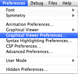
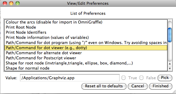
- GraphViz: in order to make use of the graphical visualization features, you need to install a version of GraphViz suitable for your architecture. Then use the command "Graphical Viewer Preferences..." in the Preferences Menu to set or check the following preferences:
- Path/Command for dot program
- Path/Command for dot viewer (e.g., dotty)
Note: you can use the "Pick" button to locate the dot program and the dot viewer. See more information about the Graphical Viewer here.
Windows Installation Instructions
Windows Specific Download Instructions
Go to the ProB Downloads site
- Go to the page Download, this should look as follows:

Install Tcl/Tk 8.5
If Tcl/Tk 8.5 is already installed you can skip this step.
- Click on the "Tcl/Tk 8.5 for Windows," link provided in the "Dependencies" column and the "Windows" row above
- Choose the most recent Tcl/Tk 8.5 distribution available for windows; be sure to choose a version matching ProB, e.g. a 32-bit version (the file highlighted in blue below) if you want to use the 32-bit version of ProB.
- Download and follow the installation instructions

Install Java
If Java 7 or newer is already installed you can skip this step.
- Click on the "Java Runtime Environment (7.0 or newer)" link provided in the "Dependencies" column and the "Windows" row above
- Follow the installation instructions
Download the ProB for Windows Zipfile
- Click on the "Zipfile (with probcli)" link in the Download column and Windows row
- Decompress and expand the ProB directory if necessary. Do not change the location and structure of the files and directories within ProB (apart from the Machines directory)! The contents of the ProB directory should look something like this:

The subfolder called "Microsoft.VC80.CRT" contains the DLLs for the Microsoft C runtime.
Optionally Download GraphViz
- Install the "dot" program and "dotty" viewer from AT&T's Graphviz package (http://www.graphviz.org/ or http://www.research.att.com/sw/tools/graphviz/)
Start ProB
- Start ProB by double-clicking on the ProBWin icon above
- Try to open some of the examples provided in the Examples folder shown above
- Contact us if you have problems
Checklist/Troubleshooting
- Java: be sure to have Java 1.7 or newer installed. Otherwise you will not be able to parse your own classical B machines as our parser is written in Java.
- Tcl/Tk: be sure to have a matching version of TclTk 8.5 installed
- In case you cannot start neither ProBWin nor probcli, you should to install the Microsoft Visual C++ 2005 Redistributable Package (x86) for yourself (rather than rely on the ones we provide in the "Microsoft.VC80.CRT" folder mentioned above).
- Try starting ProBWin or probcli from the Windows Command Prompt; the error messages may help you or us uncover the problem
- You can also try and obtain information from the main Windows Event/Error Log, by following these steps:
- Click Start, and then click Control Panel.
- Click Performance and Maintenance, then click Administrative Tools, and then double-click Computer Management. Or, open the MMC containing the Event Viewer snap-in.
- In the console tree, expand Event Viewer, and then click the log that contains the event that you want to view.
- In the details pane, double-click the event that you want to view.
- The Event Properties dialog box containing header information and a description of the event is displayed.
Editors for ProB
ProB Tcl/Tk Editor
ProB Tcl/Tk contains an editor in which syntax errors are displayed and which can be used to edit B, CSP, Z and TLA+ models. The editor of Tcl/Tk, however, has a few limitations:
- it can become very slow with long or very long lines
- the syntax highlighting can become slow with very large files. Hence, syntax highlighting is automatically turned off in some circumstances (when more than 50,000 characters are encountered or when a line is longer than 500 characters).
It is possible to open the files in an external editor. You can setup the editor to be used by modifying the preference "Path to External Text Editor" in the "Advanced Preferences" list (available in the "Preferences" menu). You can then use the command "Open FILE in external editor" in the "File" menu to open your main specification file with this editor. You can also use the command-key shortcut "Cmd-E" for this.
Launching the editor in probcli
The probcli REPL (read-eval-print-loop) supports the command :e to open the current file in the external editor, as specified in the "EDITOR" preference. You can set this preference using
probcli -repl -p EDITOR PATH
In case errors occurred with the last command, this will also try and move the cursor to the corresponding location in the file.
External Editors
VIM
A VIM plugin for ProB is available. It shows a quick fix list of parse and type errors for classical B machines (.mch) using the command line tool probcli. VIM has builtin syntax highlighting support for B.
VSCode
There is a package called B/ProB Language Support available for the VSCode editor. It adds syntax highlighting and snippets for the specification languages B and Event-B to VSCode. It integrates with probcli to obtain error markers for syntax and type errors. It can also be used for well-definedness checking.
Atom
There is a package language-b-eventb available for the Atom editor. It adds syntax highlighting and snippets for the specification languages B and Event-B to Atom. It integrates with probcli to obtain error markers for syntax and type errors.
With the Atom plugin you can now also visualize WD (well-definedness) issues in your B machines. See this small demo video.
Note that Atom is no longer being updated as of December 2022.
BBEdit
Some BBedit Language modules for B, TLA+, CSP and Prolog are available.
Emacs
A package File:B-mode.el.zip is available.
Animation
Also see the following tutorials:
- Tutorial First Step
- Tutorial Animation Tips
- Tutorial Setup Phases
- Tutorial Understanding the Complexity of B Animation
General Presentation
The ProB Main Window
The menu bar contains the various commands to access the features of ProB. It includes the traditional "File" menu with a sub-menu "Recent Files" to quickly access the files previously opened in ProB. Notice the commands "Open\Save", "Reopen\Save" and "Reopen"; the latter reopens the currently opened file and reinitializes the state of the animation and the model checking processes completely. The "About" menu provides help on the tool and includes a command to check if an update is available on the ProB website. By default, ProB starts with a limited set of commands in the Beginner mode. The Normal mode gives access to more features and can be set in the menu "Preferences|User Mode".
Under the menu bar, the main window contains four panes:
- In the top pane, the specification of the B machine is displayed with the syntax highlighted and can also be edited by typing directly in this pane; you can find out more about this editor and how to use external editors in our wiki page on editors.
- At the bottom, the animation window is composed of three panes which display at the current point during the animation:
- The current state of the B machine (State Properties), listing the current values of the machine variables;
- The enabled operations (Enabled Operations), listing the operations whose preconditions and guards are true in this state (see here for what the different colours mean);
- The history of operations leading to this state (History).
Preferences
The "Preferences" menu allows the various features of ProB to be configured. When ProB is started for the first time, it creates a file prob_preferences.pl that stores those preferences.
- The sub-menu "Font" changes the font size of the B specification displayed in the main window.
The next three commands correspond to groups of preferences displayed in separate pop-up windows.
- The command "Animation Preferences" ... configures important aspects of ProB relative to the animation and model checking of the B specifications. These preferences influence directly the way ProB interprets the B specification and are described in "Animation and Visualisation", amongst others.
- The command "Graphical Viewer Preferences" ... allows the user to set the options of the visualization tool used by ProB and the shapes and colors used to display the nodes of the state space.
- The command "Syntax Highlight Preferences" ... allows the user to activate the syntax highlight of the B specification in the main window and also to select the various colors corresponding to the syntactic elements of the B notation.
IMPORTANT: Changes in the animation preferences take effect only after reloading the machine.
Animation
| Warning This page has not yet been reviewed. Parts of it may no longer be up to date |
The animation facilities of ProB allow users to gain confidence in their specifications. These features try to be as user-friendly as possible (e.g., the user does not have to guess the right values for the operation arguments or choice variables, and he uses the mouse to operate the animation).
Basic Animation
When the B specification is opened, the syntax and type checker analyses it and, if a syntax or type error is detected, it is then reported, highlighted in yellow in the specification. Furthermore, if the B specification contains features of B that are not supported by ProB or constraints that are not satisfiable, an appropriate message is displayed. When these checks are passed, the B machine is loaded, but it has no state yet. ProB will then display the operations that can be performed in the Enabled Operations pane. These operations can be of two types described below.
Operations from the B Machine
These operations are the ones whose preconditions and guards are satisfiable in the current state. The parameter values that make true the precondition and guard are automatically computed by ProB, and one entry for the operation is displayed in the Enabled Operations pane for each group of parameter values. Each parameter value is displayed as a set between curly brackets, and the group of parameter values are enclosed between brackets after the operation name.
The computation of the parameter values greatly facilitates the work of the user, as he does not have to enumerate the possible values and check the preconditions and guards. This computation process involves trying to solve the various constraints imposed on the parameter values in the preconditions and guards.
HINT: If no operation is enabled, the state of the B machine corresponds to a deadlock
Virtual Operations
There are three particular operations that correspond to specific tasks performed by ProB:
- SETUP_CONSTANTS This virtual operation corresponds to the assignment of values to the constants of the B machine. These values must satisfy the PROPERTIES clause. ProB automatically computes the possible values and displays one initialise constants virtual operation for each possible group of of constant values. If the PROPERTIES clause is not satisfiable, an error message is displayed.
- INITIALISATION This virtual operation plays the same role as initialise constants but for initial values of the variables (clauses VARIABLES and INITIALISATION) instead of constants. If the INITIALISATION clause does not satisfy the constraints in the INVARIANT clause, an error message is displayed.
Note, there are also forward and backward buttons in the Operations pane. These enable the user to explore interactively the behaviour of the B machine.
Animating the B machine
If the B machine has constants, one or several initialise constants operations are displayed. The user selects one of these operations, then the corresponding values of the constants are displayed in the State Properties pane and the selected initialise constants operation is displayed in the History pane. In the State Properties pane, functions and relations are displayed by indicating each of their tuples on a different line.
At that point during the animation (also reached directly if the B machine has no constants), ProB displays one or several initialise machine operations. The user selects one of these operations, and then the machine is in its initial state. The initial values of the variables are displayed in the State Properties pane and the initialise machine operation selected is displayed in the History. From that moment on, an indicator of the status of the invariant is displayed at the top of the State Properties pane and the backtrack operation is displayed at the bottom of the Enabled Operations pane. The invariant status indicator is invariant ok if the invariant is satisfied or invariant violated if the invariant is violated.
From there, the user selects operations among the enabled ones. If the selected operation is backtrack, the last selected operation is removed from the top of the History pane and the previous state is displayed in the State Properties pane. If the operation was not backtrack, it is added to the History pane, the effect of the operation are computed and the state is updated in the State Properties pane
At each point during the animation process, several useful commands displaying various information on the B machine are available in the Analyse menu. The Compute Coverage command opens a window that displays three groups of information:
- NODES This is the number of nodes (i.e. states) explored so far; there are four kinds of nodes:
- live: states already computed by ProB;
- deadlocked: states where the B machine is deadlocked;
- invariant violated: states where the invariant is violated;
- open: states that are reachable from the live nodes by an enabled operation.
- COVERED OPERATIONS This is the number of operations that have been enabled so far, including the initialise machine operations.
- UNCOVERED OPERATIONS This is the names of the operations that have not been enabled so far.
The Analyse Invariant command opens a window displaying the truth values of the various conjuncts of the invariant of the B machine, while the Analyse Properties command plays the same role but for the constant properties and the Analyse Assertions plays this role for the assertions.
Animation Preferences
The animation process in ProB can be configured via several preferences set in the preference window Preferences|Animation Preferences.
First, the preference Show effect of initialisation and setup constants in operation name toggles the display of the values of the constants and the initial values of the variables when the corresponding virtual operations are shown in the Enabled Operations pane.
The preference Nr of Initialisations shown determines the number of maximum initialise machine operations that ProB should compute. Similarly, the preference Max Number of Enablings shown sets the maximum number of groups of parameter values computed for each operation of the B machine.
The preference Check invariant will toggle the display of the invariant status indicator in the State Properties pane.
Other Animation Features
Several other commands are provided by ProB in the Animate menu for animating B specifications. The Reset command will set the state of the machine to the root, as if the machine has just been opened, i.e. when the initialise constants or initialise machine operations are displayed in the Enabled Operations pane. The Random Animation(10) command operates a sequence of 10 randomly chosen operations from the B specification. The variant Random Animation enables to specify the number of operation to operate randomly. In the File menu, the command Save State stores the current state of the B machine, which can then be reloaded with the command Load Saved State.
Colours of enabled operations
The enabled operations are shown in different colours, depending on the state where the operation leads to. If more than one rule of the following list apply, the first colour is taken:
- blue
- The operation does not change the state (behaves like skip).
- green
- The operation leads to a new, not yet explored state.
- red
- The operation leads to a state where the invariant is violated.
- orange
- The operation leads to a deadlock state, i.e. a state where no operation is enabled.
- black
- Otherwise, the operation leads to a state that is different to the current state, has already been visited and is neither an invariant violating or deadlock state.
Controlling ProB Preferences
ProB provides a variety of preferences to control its behaviour. A list of the most important preferences can be found in the manual page for probcli. We also have a separate manual page about setting the sizes of deferred sets.
Setting Preferences in a B machine
This only works for classical B models. For a preference P you can add the following definition to the DEFINITIONS section of the main machine:
SET_PREF_P == VAL
This will set the preference P to the value VAL for this model only.
Setting Preferences from the command-line
You can set a preference P to a value VAL for a particular run of probcli by adding the command-line switch -p P VAL, e.g.,
probcli -p P VAL mymachine.mch -mc 9999
You can obtain a list of preferences by calling probcli as follows:
probcli -help -v
You can use a preference file generated by ProB Tcl/Tk:
-prefs FILE
This will import all preferences from this file, as set by ProB Tcl/Tk.
You can also set the scope for a particular deferred set GS using the following command-line switch:
-card GS Val
Setting Preferences from ProB Tcl/Tk
ProB Tcl/Tk stores your preferences settings in a file ProB_Preferences.pl.
The ProB preferences are grouped into various categories. In the "Preferences" Menu you can modify the preferences for each category:

For example, if you choose the graphical viewer preferences you will get this dialog:

B Language
Current Limitations
ProB in general requires all deferred sets to be given a finite cardinality. If no cardinality is specified, a default size will be used. Also, unless finite bounds can be inferred by the ProB constraint solver, mathematical integers will only be enumerated within MININT to MAXINT (and ProB will generate enumeration warnings in case no solution is found).
Other general limitations are:
- Trees and binary trees. These constructs are specific to the AtelierB tool and are only partially supported;
- Definitions. Definitions (from the DEFINITIONS clause) with arguments are supported, but in contrast to AtelierB they are parsed independently and have to be either an expression, a predicate, or a substitution; definitions which are predicates or substitutions must be declared before first use. Also: the arguments of DEFINITIONS have to be expressions. Finally, when replacing DEFINITIONS the associativity is not changed. E.g., with PLUS(x,y) == x+y, the expression PLUS(2,3)*10 will evaluate to 50 (and not to 32 as with Atelier-B).
Also, ProB will generate a warning when variable capture may occur.
- There are also limitations with refinements. See below;
- VALUES This clause of IMPLEMENTATION machines is not yet fully supported;
- Parsing: ProB will require parentheses around the comma, the relational composition, and parallel product operators. For example, you cannot write r2=rel;rel. You need to write r2=(rel;rel). This allows ProB to distinguish the relational composition from the sequential composition (or other uses of the semicolon). You also generally need to put BEGIN and END around the sequential composition operator, e.g., Op = BEGIN x:=1;y:=2 END.
See the page Using ProB with Atelier B for more details.
Multiple Machines and Refinements
It is possible to use multiple classical B machines with ProB. However, ProB may not enforce all of the classical B visibility rules (although we try to). As far as the visibility rules are concerned, it is thus a good idea to check the machines in another B tool, such as Atelier B or the B-Toolkit.
While refinements are supported, the preconditions of operations are not propagated down to refinement machines. This means that you should rewrite the preconditions of operations (and, if necessary, reformulate them in terms of the variables of the refinement machine). Also, the refinement checker does not yet check the gluing invariant.
Note however, that for Rodin Event-B models we now support multi-level animation and validation.
Summary of B Syntax
Summary of B Syntax
Below we describe the "classical" B syntax as supported by ProB. You may also wish to consult
- The B summary by Ken Robinson (File:B-summary.pdf)
- The Atelier-B reference manual (b-language-reference-manual.pdf)
Logical predicates
 P & Q        conjunction
 P or Q       disjunction
 P => Q       implication
 P <=> Q      equivalence
 not(P)       negation
 !(x).(P=>Q)  universal quantification
 #(x).(P&Q)   existential quantification
 btrue        truth (this is a predicate)
 bfalse       falsity (this is a predicate)
Above, P and Q stand for predicates. Inside the universal quantification, P must give a value type to the quantified variable. Note: you can also introduce multiple variables inside a universal or existential quantification, e.g., !(x,y).(P => Q).
Equality
 E = F   equality
 E /= F  disequality
Booleans
 TRUE     truth value (this is an expression)
 FALSE    falsity value (this is an expression)
 BOOL     set of boolean values ({TRUE,FALSE})
 bool(P)  convert predicate into BOOL value
Warning: TRUE and FALSE are expression values and not predicates in B and cannot be combined using logical connectives. To combine two boolean values x and y using conjunction you have to write x=TRUE & y=TRUE. To convert a predicate such as z>0 into a boolean value you have to use bool(z>0).
Sets
 {}              empty set
 {E}             singleton set
 {E,F}           set enumeration
 {x|P}           comprehension set
 {(x).P|E}       Event-B style comprehension set (brackets needed)
 POW(S)          power set
 POW1(S)         set of non-empty subsets
 FIN(S)          set of all finite subsets
 FIN1(S)         set of all non-empty finite subsets
 card(S)         cardinality
 S*T             cartesian product
 S\/T            set union
 S/\T            set intersection
 S-T or S \ T    set difference
 E:S             element of
 E/:S            not element of
 S<:T            subset of
 S/<:T           not subset of
 S<<:T           strict subset of
 S/<<:T          not strict subset of
 union(S)        generalised union over sets of sets
 inter(S)        generalised intersection over sets of sets
 UNION(z).(P|E)  generalised union with predicate
 INTER(z).(P|E)  generalised intersection with predicate
Integers
 INTEGER         set of integers
 NATURAL         set of natural numbers
 NATURAL1        set of non-zero natural numbers
 INT             set of implementable integers (MININT..MAXINT)
 NAT             set of implementable natural numbers
 NAT1            set of non-zero implementable natural numbers
 n..m            set of numbers from n to m
 MININT          the minimum implementable integer
 MAXINT          the maximum implementable integer
 m>n             greater than
 m<n             less than
 m>=n            greater than or equal
 m<=n            less than or equal
 max(S)          maximum of a set of numbers
 min(S)          minimum of a set of numbers
 m+n             addition
 m-n             difference
 m*n             multiplication
 m/n             division
 m**n            power
 m mod n         remainder of division
 PI(z).(P|E)     set product
 SIGMA(z).(P|E)  set summation
 succ(n)         successor (n+1)
 pred(n)         predecessor (n-1)
 0xH             hexadecimal literal, where H is a sequence of letters in [0-9A-Fa-f]
Relations
 S<->T         relation
 S<<->T        total relation
 S<->>T        surjective relation
 S<<->>T       total surjective relation
 E|->F         maplet
 dom(r)        domain of relation
 ran(r)        range of relation
 id(S)         identity relation
 S<|r          domain restriction
 S<<|r         domain subtraction
 r|>S          range restriction
 r|>>S         range subtraction
 r~            inverse of relation
 r[S]          relational image
 r1<+r2        relational overriding (r2 overrides r1)
 r1><r2        direct product (all pairs (x,(y,z)) with x,y:r1 and x,z:r2)
 (r1;r2)       relational composition {x,y| x|->z:r1 & z|->y:r2}
 (r1||r2)      parallel product (all pairs ((x,v),(y,w)) with x,y:r1 and v,w:r2)
 prj1(S,T)     projection function (usage prj1(Dom,Ran)(Pair))
 prj2(S,T)     projection function (usage prj2(Dom,Ran)(Pair))
               prj1(Pair) and prj2(Pair) are also allowed
 fnc(r)        translate relation A<->B into function A+->POW(B)
 rel(r)        translate relation A<->POW(B) into relation A<->B
 closure1(r)   transitive closure
 closure(r)    reflexive & transitive closure
               (equal to id(TYPEOF_r) \/ closure1(r))
 iterate(r,n)  iteration of r with n>=0
               (Note: iterate(r,0)=id(s) where s=TYPEOF_r)
Functions
 S+->T         partial function
 S-->T         total function
 S+->>T        partial surjection
 S-->>T        total surjection
 S>+>T         partial injection
 S>->T         total injection
 S>+>>T        partial bijection
 S>->>T        total bijection
 %x.(P|E)      lambda abstraction
 f(E)          function application
 f(E1,...,En)  is also supported (as well as f(E1|->E2...|->En))
Sequences
 [] or <>  empty sequence
 [E]       singleton sequence
 [E,F]     constructed sequence
 seq(S)    set of sequences over S
 seq1(S)   set of non-empty sequences over S
 iseq(S)   set of injective sequences over S
 iseq1(S)  set of non-empty injective sequences over S
 perm(S)   set of bijective sequences (permutations) over S
 size(s)   size of sequence
 s^t       concatenation
 E->s      prepend element
 s<-E      append element
 rev(s)    reverse of sequence
 first(s)  first element
 last(s)   last element
 front(s)  front of sequence (all but last element)
 tail(s)   tail of sequence (all but first element)
 conc(S)   concatenation of sequence of sequences
 s/|\n     take first n elements of sequence
 s\|/n     drop first n elements from sequence
Records
 struct(ID:S,...,ID:S)  set of records with given fields and field types
 rec(ID:E,...,ID:E)     construct a record with given field names and values
 E'ID                   get value of field with name ID
Identifiers
 ID    must start with letter (ASCII or Unicode), can then contain
       letters (ASCII or Unicode), digits and underscore (_) and
       can end with Unicode subscripts followed by Unicode primes
 M.ID  composed identifier for identifier coming from included machine M
 `ID`  an identifier in backquotes can contain almost any character (except newline)
Strings
 "astring"      a specific (single-line) string value
 '''astring'''  an alternate way of writing (multi-line) strings, no need to escape "
 ```tstring```  template strings, where ${Expr} parts are evaluated and converted to string,
                you can provide options separated by commas in square brackets like $[2f]{Expr}.
                Valid options are: Nf (for floats/reals), Nd (for integer), Np (padding),
                ascii (can be abbreviated to a), unicode (can be abbreviated to u).
 STRING         the set of all strings
Atelier-B does not support any operations on strings, apart from equality and disequality. In ProB, however, some of the sequence operators work also on strings:
 size(s)   the length of a string s
 rev(s)    the reverse of a string s
 s ^ t     the concatenation of two strings
 conc(ss)  the concatenation of a sequence of strings
You can turn this support off using the STRING_AS_SEQUENCE preference. The library LibraryStrings.def in stdlib contains additional useful external functions (like TO_STRING, STRING_SPLIT, FORMAT_TO_STRING, INT_TO_HEX_STRING, ...).
ProB also allows multi-line strings.
As of version 1.7.0, ProB will support the following escape sequences within strings:
 \n  newline (ASCII character 13)
 \r  carriage return (ASCII 10)
 \t  tab (ASCII 9)
 \"  the double quote symbol "
 \'  the single quote symbol '
 \\  the backslash symbol
Within single-line string literals, you do not need to escape '. Within multi-line string literals, you do not need to escape " and you can use tabs and newlines.
ProB assumes that all B machines and strings use the UTF-8 encoding.
Reals
 REAL        set of reals
 FLOAT       set of floating point numbers
 i.f         real literal in decimal notation, where i and f are natural numbers
 i.fEg       real literal in scientific notation, where i,f are natural numbers and g is an integer
 real(n)     convert an integer n into a real number
 floor(r)    convert a real r into an integer
 ceiling(r)  convert a real r into an integer
One can also use a lowercase e for literals in scientific notation (e.g. 1.0e-10). Standard arithmetic operators can be applied to reals: +, - , *, /, SIGMA, PI. Exponentiation of a real with an integer is also allowed. The comparison predicates =, /=, <, >, <=, >= also all work. Support for reals and floats is experimental. The definition in Atelier-B is also not stable yet. Currently ProB supports floating point numbers only. Warning: properties such as associativity and commutativity of arithmetic operators thus do not hold. The library LibraryReals.def in stdlib contains additional useful external functions (like RSIN, RCOS, RLOG, RSQRT, RPOW, ...). You can turn off support for REALS using the preference ALLOW_REALS. The REAL_SOLVER preference how constraints are solved.
Trees
Nodes in the tree are denoted by index sequences (branches), e.g, n=[1,2,1] Each node in the tree is labelled with an element from a domain S. A tree is a function mapping of branches to elements of the domain S.
 tree(S)       set of trees over domain S
 btree(S)      set of binary trees over domain S
 top(t)        top of a tree
 const(E,s)    construct a tree from info E and sequence of subtrees s
 rank(t,n)     rank of the node at end of branch n in the tree t
 father(t,n)   father of the node denoted by branch n in the tree t
 son(t,n,i)    the ith son of the node denoted by branch n in tree t
 sons(t)       the sequence of sons of the root of the tree t
 subtree(t,n)
 arity(t,n)
 bin(E)        construct a binary tree with a single node E
 bin(tl,E,tr)  construct a binary tree with root info E and subtrees tl,tr
 left(t)       the left (first) son of the root of the binary tree t
 right(t)      the right (last) son of the root of the binary tree t
 sizet(t)      the size of the tree (number of nodes)
 prefix(t)     the nodes of the tree t in prefix order
 postfix(t)    the nodes of the tree t in prefix order
 mirror, infix are recognised by the parser but not yet supported by ProB itself
LET and IF-THEN-ELSE
ProB allows the following for predicates, expressions and substitutions:
 IF P THEN E1 END                    conditional branching
 IF P THEN E1 ELSIF E2 END           we also allow multiple ELSIF branches
 IF P THEN E1 ELSE E2 END            but you always need an ELSE branch for expressions and predicates
 IF P THEN E1 ELSIF E2 ELSE E3 END
 LET x1,... BE x1=E1 & ... IN E END  introduce local variables
Note: the expression Ei defining xi is allowed to use x1,...,x(i-1) for predicates/expressions. By setting the preference ALLOW_COMPLEX_LETS to TRUE, this is also allowed for substitutions.
Statements (aka Substitutions)
 skip                                                      no operation
 x := E                                                    assignment
 f(x) := E                                                 functional override
 x :: S                                                    choice from set
 x : (P)                                                   choice by predicate P (constraining x; previous value of x is x$0)
 x <-- OP(x)                                               call operation and assign return value
 G||H                                                      parallel substitution**
 G;H                                                       sequential composition**
 ANY x,... WHERE P THEN G END                              non deterministic choice
 LET x,... BE x=E & ... IN G END
 VAR x,... IN G END                                        generate local variables
 PRE P THEN G END
 ASSERT P THEN G END
 CHOICE G OR H END
 IF P THEN G END
 IF P THEN G ELSE H END
 IF P1 THEN G1 ELSIF P2 THEN G2 ... END
 IF P1 THEN G1 ELSIF P2 THEN G2 ... ELSE Gn END
 SELECT P THEN G WHEN ... WHEN Q THEN H END
 SELECT P THEN G WHEN ... WHEN Q THEN H ELSE I END
 CASE E OF EITHER m THEN G OR n THEN H ... END END
 CASE E OF EITHER m THEN G OR n THEN H ... ELSE I END END
 WHILE P1 DO G INVARIANT P2 VARIANT E END
 WHEN P THEN G END                                         is a synonym for SELECT P THEN G END
**: cannot be used at the top-level of an operation, but needs to be wrapped inside a BEGIN END or another statement (to avoid confusion with the operators ; and || on relations).
Machine header
MACHINE or REFINEMENT or IMPLEMENTATION
Note: machine parameters can either be SETS (if identifier is all upper-case) or scalars (i.e., integer, boolean or SET element; if identifier is not all upper-case; typing must be provided be CONSTRAINTS)
You can also use MODEL or SYSTEM as a synonym for MACHINE, as well as EVENTS as a synonym for OPERATIONS. ProB also supports the ref keyword of Atelier-B for event refinement.
Machine sections
 CONSTRAINTS         P                     (logical predicate)
 SETS                S;T={e1,e2,...};...
 FREETYPES           x=x1,x2(arg2),...;...
 CONSTANTS           x,y,...
 CONCRETE_CONSTANTS  cx,cy,...
 PROPERTIES          P                     (logical predicate)
 DEFINITIONS         m(x,...) == BODY;...
 VARIABLES           x,y,...
 CONCRETE_VARIABLES  cv,cw,...
 INVARIANT           P                     (logical predicate)
 ASSERTIONS          P;...;P               (list of logical predicates separated by ;)
 INITIALISATION      S                     (substitution)
 OPERATIONS          O;...                 (operations)
Machine inclusion
 USES      list of machines
 INCLUDES  list of machines
 SEES      list of machines
 EXTENDS   list of machines
 PROMOTES  list of operations
 REFINES   machine
Note: Refinement machines should express the operation preconditions in terms of their own variables.
Definitions
 NAME1 == Expression;     Definition without arguments
 NAME2(ID,...,ID) == E2;  Definition with arguments
 "FILE.def";              Include definitions from file
There are a few specific definitions which can be used to influence ProB:
 GOAL == P                          to define a custom Goal predicate for Model Checking
                                    (the Goal is also set by using "Advanced Find...")
 SCOPE == P                         to limit the search space to "interesting" nodes
 scope_SETNAME == n..n              to define custom cardinality for set SETNAME
 scope_SETNAME == n                 equivalent to 1..n
 SET_PREF_MININT == n
 SET_PREF_MAXINT == n
 SET_PREF_MAX_INITIALISATIONS == n  max. number of intialisations computed
 SET_PREF_MAX_OPERATIONS == n       max. number of enablings per operation computed
 MAX_OPERATIONS_OPNAME == n         max. number of enablings for the operation OPNAME
 SET_PREF_SYMBOLIC == TRUE/FALSE
 SET_PREF_TIME_OUT == n             time out for operation computation in ms
 ASSERT_LTL... == "LTL Formula"  	using X,F,G,U,R LTL operators +
                                    Y,O,H,S Past-LTL operators +
                                    atomic propositions: e(OpName), [OpName], {BPredicate}
 HEURISTIC_FUNCTION == n            in directed model-checking mode nodes with smalles value will be processed first
The following definitions allow providing a custom state visualization (n can be empty or a number):
 ANIMATION_FUNCTIONn == e                           a function (INT*INT) +-> INT or an INT
 ANIMATION_FUNCTION_DEFAULT == e                    a function (INT*INT) +-> INT or an INT
                                                    instead of any INT above you can also use BOOL or any SET
                                                    as a result you can also use STRING values,
                                                    or even other values which are pretty printed
 ANIMATION_IMGn == "PATH to .gif"                   a path to a gif file
 ANIMATION_STRn == "sometext"                       a string without spaces;
                                                    the result integer n will be rendered as a string
 ANIMATION_STR_JUSTIFY_LEFT == TRUE                 computes the longest string in the outputs and pads
                                                    the other strings accordingly
 SET_PREF_TK_CUSTOM_STATE_VIEW_PADDING == n         additional padding between images in pixels
 SET_PREF_TK_CUSTOM_STATE_VIEW_STRING_PADDING == n  additional padding between text in pixels
The following definitions allow providing a custom state graph (n can be empty or a number):
 CUSTOM_GRAPH_NODESn == e  define a set of nodes to be shown,
                           nodes can also be pairs (Node,Colour), triples (Node,Shape,Colour) or
                           records or sets of records like
                           rec(color:Colour, shape:Shape, style:Style, label:Label, value:Node, ...)
                           Colours are strings of valid Dot/Tk colors (e.g., "maroon" or "red")
                           Shapes are strings of valid Dot shapes (e.g., "rect" or "hexagon"), and
                           Styles are valid Dot shape styles (e.g., "rounded" or "solid" or "dashed")
 CUSTOM_GRAPH_EDGESn == e  define a relation to be shown as a graph
                           edges can either be pairs (node1,node2) or triples (node1,Label,node2)
                           where Label is either a Dot/Tk color or a string or value representing
                           the label to be used for the edges
In both cases e can also be a record which defines default dot attributes like color, shape, style and description, e.g.:
 CUSTOM_GRAPH_NODES == rec(color:"blue", shape:"rect", style:"filled", nodes:e);
 CUSTOM_GRAPH_EDGES == rec(color:"red", style:"dotted", dir:"none", penwidth:2, edges:e)
Alternatively, the complete graph can be put into one definition using CUSTOM_GRAPH.
You have to define a single CUSTOM_GRAPH definition of a record with global graph attributes
  (like rankdir or layout) and optionally with edges and nodes attributes (replacing
   CUSTOM_GRAPH_EDGES and CUSTOM_GRAPH_NODES respectively), e.g.:
CUSTOM_GRAPH == rec(layout:"circo", nodes:mynodes, edges:myedges)
You can now also use a single CUSTOM_GRAPH definition of a record with global graph attributes (like rankdir or layout) and optionally with edges and nodes attributes (replacing CUSTOM_GRAPH_EDGES and CUSTOM_GRAPH_NODES respectively), e.g.:
CUSTOM_GRAPH == rec(layout:"circo", nodes:mynodes, edges:myedges)
You can also provide SEQUENCE_CHART_opname definitions for generating UML sequence charts.
These DEFINITIONS affect VisB:
 VISB_JSON_FILE == "PATH to .json"  a path to a default VisB JSON file for visualisation;
                                    if it is "" an empty SVG will be created
 VISB_SVG_OBJECTSn == ...           define a record or set of records for creating new SVG objects
 VISB_SVG_UPDATESn == ...           define a record or set of records containing updates of SVG objects
 VISB_SVG_HOVERSn == ...            define a record or set of records for VisB hover functions
 VISB_SVG_BOX == ...                record with dimensions (height, width) of a default empty SVG
 VISB_SVG_CONTENTS == ...           defines a string to be included into a created empty SVG file
Comments and Pragmas
B supports two styles of comments:
 /* ... */  block comments
 // ...     line comments
ProB recognises several pragma comments of the form /*@ PRAGMA VALUE */ The whitespace between @ and PRAGMA is optional.
 /*@symbolic */             put before comprehension set, lambda, union or composition to instruct ProB
                            to keep it symbolic and not try to compute it explicitly
 /*@label LBL */            associates a label LBL with the following predicate
                            (LBL must be identifier or a string "....")
 /*@desc DESC */            associates a description DESC with the preceding predicate or
                            introduced identifier (in VARIABLES, CONSTANTS,... section)
                            There are three special descriptions:
                            /*@desc memo*/          to be put after identifiers in the ABSTRACT_CONSTANTS section
                                                    indicating that these functions should be memoized
                            /*@desc expand*/        to be put after identifiers (in VARIABLES, CONSTANTS,... section)
                                                    indicating that they should be expanded and not kept symbolically
                            /*@desc prob-ignore */  to be put after predicates (e.g., in PROPERTIES) which
                                                    should be ignored by ProB
                                                    when the preference USE_IGNORE_PRAGMAS is TRUE
 /*@file PATH */            associates a file for machines in SEES, INCLUDES, ...
                            put pragma after a seen or included machine
 /*@package NAME */         at start of machine, machine file should be in folder NAME/...
                            NAME can be qualified N1.N2...Nk, in which case the machine
                            file should be in N1/N2/.../Nk
 /*@import-package NAME */  adds ../NAME to search paths for SEES,...
                            NAME can also be qualified N1.N2...Nk, use after package pragma
 /*@generated */            can be put at the top of a machine file; indicates the machine
                            is generated from some other source
File Extensions
 .mch   for abstract machine files
 .ref   for refinement machines
 .imp   for implementation machines
 .def   for DEFINITIONS files
 .rmch  for Rules machines for data validation
Free Types
More information can be found here.
Free types exist in Z and in the Rodin theory plugin and are supported by ProB. You can also define new free types in classical B by adding a FREETYPES clause with free type definitions separated by semicolon.
Here is a definition of an inductive type IntList for lists of integers constructed using inil and icons:
FREETYPES
  IntList = inil, icons(INTEGER*IntList)
Differences with AtelierB/B4Free
Basically, ProB tries to be compatible with Atelier B and conforms to the semantics of Abrial's B-Book and of Atelier B's reference manual. Here are the main differences with Atelier B:
 - tuples without parentheses are not supported; write (a,b,c) instead of a,b,c
 - relational composition has to be wrapped into parentheses; write (f;g)
 - parallel product also has to be wrapped into parentheses; write (f||g)
 - not all tree operators are supported
 - the VALUES clause is only partially supported
 - definitions have to be syntactically correct and be either an expression,
   predicate or substitution;
   the arguments to definitions have to be expressions;
   definitions which are predicates or substitutions must be declared before first use
 - definitions are local to a machine
 - for ProB the order of fields in a record is not relevant (internally the fields are
   sorted), Atelier-B reports a type error if the order of the name of the fields changes
 - well-definedness: for disjunctions and implications ProB uses the L-system
   of well-definedness (i.e., for P => Q, P should be well-defined and
   if P is true then Q should also be well-defined)
 - ProB allows WHILE loops and sequential composition in abstract machines
 - ProB now allows the IF-THEN-ELSE and LET for expressions and predicates
   (e.g., IF x<0 THEN -x ELSE x END or LET x BE x=f(y) IN x+x END)
 - ProB's type inference is stronger than Atelier-B's, much less typing predicates
   are required
 - You can apply prj1 and prj2 without providing the type arguments, e.g., prj2(prj1(1|->2|->3))
 - ProB accepts operations with parameters but without pre-conditions
 - ProB allows identifiers consisting of a single character and identifiers in single backquotes (`id`)
 - ProB allows to use <> for the empty sequence (but this use is deprecated)
 - ProB allows escape codes (\n, \', \", see above) and supports UTF-8 characters in strings,
   and ProB allows multi-line string literals written using three apostrophes ('''string''')
   as well as template strings using three backquotes (e.g., ```1+2=${1+2}```)
 - ProB allows a she-bang line in machine files starting with #!
 - ProB allows btrue and bfalse as predicates in B machines
 - ProB allows to use the Event-B relation operators <<->, <->>, <<->>
 - ProB allows set comprehensions with an extra expression like {x•x:1..10|x*x}.
 - The FREETYPES section and the external libraries (LibraryStrings.def, ...) do not exist in Atelier-B
See also our Wiki for documentation:
Also note that there are various differences between BToolkit and AtelierB/ProB:
 - AtelierB/ProB do not allow true as predicate;
   e.g., PRE true THEN ... END is not allowed (use BEGIN ... END instead)
   ProB now allows btrue and bfalse to be used as predicates.
 - AtelierB/ProB do not allow a machine parameter to be used in the PROPERTIES
 - AtelierB/ProB require a scalar machine parameter to be typed in the
   CONSTRAINTS clause
 - In AtelierB/ProB the BOOL type is pre-defined and cannot be redefined
If you discover more differences, please let us know!
Other notes
 ProB now supports the Unicode mathematical symbols, exactly like Atelier-B
 ProB is best at treating universally quantified formulas of the form
   !x.(x:SET => RHS), or
   !(x,y).(x|->y:SET =>RHS),
   !(x,y,z).(x|->y|->z:SET =>RHS), ...;
 otherwise the treatment of !(x1,...,xn).(LHS => RHS) may delay until all values
 treated by LHS are known.
 Similarly, expressions of the form SIGMA(x).(x:SET|Expr) and PI(x).(x:SET|Expr)
 lead to better constraint propagation.
 The construction S:FIN(S) is recognised by ProB as equivalent to the Event-B
 finite(S) operator.
 ProB assumes that machines and STRING values are encoded using UTF-8.
Event-B Syntax
Note that the Event-B syntax in Rodin is slightly different (e.g, no sequences or strings built-in). There is also an Event-B summary by Ken Robinson (File:EventB-summary.pdf). The Event-B syntax is only available for Event-B models in Rodin, ProB2-UI and ProB Jupyter notebooks.
Feedback
Please help us to improve this documentation by providing feedback in our bug tracker, asking questions in our prob-users group or sending an email to Michael Leuschel.
Types
| Warning This page has not yet been reviewed. Parts of it may no longer be up to date |
ProB requires all constants and variables to be typed. As of version 1.3, ProB uses a new unification-based type inference and checking algorithm. As such, you should be able to use most Atelier B models without problem. On the other hand, certain models that ProB accepts will have to be rewritten to be type checked by Atelier B (e.g., by adding additional typing predicates). Also note that, in contrast to Atelier B, ProB will type check macro DEFINITIONS.
What is a basic type in B
- BOOL
- INTEGER
- Any name of a set introduced in a SETS clause or introduced as a parameter of the machine
- POW (τ) (power set) for τ being a type
- τ1 * τ2 (Cartesian product) for τ1 and τ2 being two types
What needs to be typed
Generally speaking, any constant or variable. More precisely:
- Constants declared in the CONSTANTS clause must be typed in the PROPERTIES clause;
- Variables declared in the VARIABLES clause must be typed in the INVARIANT;
- Arguments of an operation must be typed in the precondition PRE or a top-level SELECT statement of the operation;
- Variables in universal or existential quantifications;
- Variables of set comprehensions must be typed in a conjunct of the body of the set comprehension. For example, {xx | xx:NAT & xx>0 & xx<5} is fine, but {xx | xx>0 & xx<5} is not;
- Variables of lambda abstractions must be typed in the predicate part of the abstraction. For example, %yy.(yy:NAT|yy-1) properly types the variable yy;
- Variables introduced in ANY statements must be typed in the WHERE part of the statement.
ProB will warn you if a variable has not been given a type.
HINT: The Analyse|Show Typing command reveals the typing that ProB has inferred for your constants and global variables.
Restriction on the Domains of the Variables
Animating and verifying a B specification is in principle undecidable. ProB overcomes this by requiring that the domain of the variables is finite (i.e., with finitely many values) or integer. This ensures that the state space has finite size. Typing of the B specification ensures this restriction.
In the B specification, a set is either defined explicitely, thus being a finite domain, or its definition is deferred. In the later case, the user can indicate the size of the set mySET (without defining its elements) by creating a macro in the DEFINITIONS clause with the name scope_mySET and an integer value (e.g. scope_mySET==2) or a value specified as a range (e.g. scope_mySET == 1..12). The macros with the prefix "scope_" will be used by ProB and do not modify the B specification. If the size of the set is unspecified, ProB considers the set to have a default size. The value for the default size is defined in the Preferences|Animation Preferences... preference window by the preference Size of unspecified sets in SETS section.
The B method enables to specify the size of a set with the card operator in the PROPERTIES clause; this form of constraint is now supported by ProB, provided it is of a simple form card(S)=Nr, where S is a deferred set and Nr a natural number.
Enumeration in ProB
The typing information is used by ProB to enumerate the possible values of a constant or a variable whenever a specification does not narrow down that value to a single value.
For example, if you write xx:NAT & xx=1 ProB does not have to resort to enumeration as the xx=1 constraint imposes a single possible value for xx. However, if you write xx:NAT & xx<3 ProB will enumerate the possible values of xx in order to find those that satisfy the constraints imposed by the machine (here 0,1,2).
ProB will use the constraints to try to cut down the enumeration space, and will resort to enumeration usually only as a last resort. So something like xx:NAT & xx<10 & x>2 & x=5 will not result in enumeration.
The enumeration range for integers is controlled by two preferences in the Preferences|Animation Preferences... preference window: !MinInt, used for expressions such as xx::INT, and !MaxInt, used for expressions such as xx::NAT preferences. Nevertheless, writing xx: NAT & xx = 55 puts the value 55 in x no matter what !MaxInt is set to, as no enumeration is required.
Note that these preferences also apply to the mathematical integers (INTEGER) and natural numbers (NATURAL). In case a mathematical integer or natural number is enumerated (using !MinInt and !MaxInt) a warning is printed on the console.
Deferred Sets
A deferred set in B is declared in the SETS Section and is not explicitly enumerated. In the example below, AA is a deferred set and BB is an enumerated set.
MACHINE M0
SETS AA; BB={bb,cc,dd}
END
ProB in general requires all deferred sets to be given a finite cardinality before starting animation or model checking. If no cardinality is specified, a default size will be used (which is controlled by the DEFAULT_SETSIZE preference).
In general (for both probcli and ProB Tcl/Tk) you can set the cardinality of a set AA either by
- making it an enumerated set, i.e., adding AA = {v1,v2,…} to the SETS clause
- adding a predicate card(AA) = constant to the PROPERTIES clause
- Note: various other predicates in the PROPERTIES clause will also influence the size used for AA by ProB, for example:
     - card(AA) > 1
     - aa:AA & bb:AA & aa/=bb
     - AA = {aa,bb} & aa/=bb
     - …
- you can add a DEFINITION scope_AA == constant to instruct ProB to set the cardinality of AA to the constant.
Using Refinement for Animation Preferences
Note: instead of adding AA = {aa,bb} to the SETS clause you can also add AA = {aa,bb} & aa/=bb to the PROPERTIES clause. This can also be done in a refinement. A good idea is then to generate a refinement for animation with ProB (which may contain other important settings for animation):
REFINEMENT M0_ProB REFINES M0
CONSTANTS aa,bb
PROPERTIES
AA = {aa,bb} & aa/=bb
END
Setting Deferred Set Cardinalities within probcli
From the command-line, using probcli you can use the command-line switch:
-card <GS> <VAL>
Example:
probcli my.mch -card PID 5
Free Types
Summary
Free types exist in Z and in the Rodin theory plugin and are supported by ProB. You can also define new free types in classical B by adding a FREETYPES clause with free type definitions separated by semicolon.
Here is a definition of an inductive type IntList for lists of integers constructed using inil and icons:
FREETYPES
  IntList = inil, icons(INTEGER*IntList)
What is a Free Type
Free types are sum types [4]. They make it easier to define recursive structures. A free type value may take exactly one of the defined subtypes, with additional payload data, and later the exact subtype can be queried and the payload data retrieved.
Syntax
FREETYPES
The FREETYPES machine clause contains a semicolon separated list of Freetype Definitions:
FREETYPES
  <Freetype Definition 1>;
  ...;
  <Freetype Definition N>
Freetype Definition
Each Freetype Definition consists of an identifier (the name of the free type), followed by an equals symbol and one or more Freetype Constructors separated by commas:
<Identifier> = <Freetype Constructor 1>, ..., <Freetype Constructor N>
Freetype Constructor
A Freetype Constructor may be a single identifier (the name of the free type constructor) or an identifier with a single expression argument (the type of the payload data) in parentheses.
<Identifier>
<Identifier>(<Expression>)
Semantics
The name of the free type can be used anywhere in the machine as a type identifier (like a set) to define the type of a value.
To actually create a value of the free type one needs to use one of the free type constructors. Free type constructors that do not take an argument can be used as the right side of an assignment as-is, while free type constructors that have an argument need a value parameter of that type - this works like a function call. Because those constructor calls work like function calls, we benefit from the tuple-function syntactic sugar and can use one tuple parameter as a way to represent multiple logical parameters and call the constructor with values separated by commas without having to create a tuple first.
Internally constructors without parameter are just values, while constructors with parameters are functions that take the payload data and return the free type value with the given payload. To check whether a free type value has a specific subtype one can use equality for parameter-less constructors and membership in the range for constructors with a parameter.
To get the contained value out of a free type value one can use the inverse constructor (also called deconstructor), simply created by applying the B operator ~.
Example
In our example from the introduction we have a free type with two constructors that represents a list. The constructor inil represents an empty list and takes no argument, while the icons constructor represents a list head with the first value and the rest of the list combined as a tuple.
To create a list with content we are using the simplified function call syntax, so we do not have to construct the tuple (head, tail) directly.
To get values out of the icons subtype we use the the deconstructor icons~. The resulting value is a tuple which we need to project to the first or second value respectively.
Here we implement a stack:
MACHINE IntListTest
FREETYPES IntList = inil, icons(INTEGER*IntList)
VARIABLES list
INVARIANT list : IntList
INITIALISATION list := inil
OPERATIONS
    push(value) = PRE value : INTEGER THEN
        list := icons(value, list)
    END;
    pop = PRE list /= inil THEN
        list := prj2(icons~(list))
    END;
    value <-- peek = PRE list : ran(icons) THEN
        value := prj1(icons~(list))
    END
END
Example usage in ProB2-UI:

External Functions
As of version 1.3.5-beta7 ProB can make use of externally defined functions. These functions must currently be written in Prolog (in principle C, Java, Tcl or even other languages can be used via the SICStus Prolog external function interfaces). These functions can be used to write expression, predicates, or substitutions. The general mechanism that is used is to mark certain DEFINITIONS as external, in which case ProB will make use of external Prolog code rather than using the right-hand-side of the DEFINITION whenever it is used. However, these DEFINITIONS can often (unless they are polymorphic) be wrapped into B (constant) functions. If you just want to use the standard external functions already defined by ProB, then you don't have to understand this mechanism in detail (or at all).
We have a PDF describing the external functions generated from a ProB-Jupyter notebook: File:ExternalFunctions.pdf The Notebook is available and can now be launched via binder.
Standard Libraries provided by ProB
In a first instance we have predefined a series of external functions and grouped them in various library machines and definition files:
- LibraryMath.mch: defining sin, cos, tan, sinx, cosx, tanx, logx, gcd, msb, random as well as access to all other Prolog built-in arithmetic functions.
- LibraryStrings.mch: functions manipulating B STRING objects by providing length, append, split and conversion functions chars, codes.
- LibraryStrings.def used by LibraryStrings.mch: providing direct access to various operators on strings (STRING_LENGTH, STRING_APPEND, STRING_SPLIT INT_TO_STRING,...)
- LibraryFiles.mch: various functions to obtain information about files and directories in the underlying file system
- LibraryIO.def: providing functions to write information to screen or file. Note: these external functions are polymorphic and as such cannot be defined as B constants: you have to use the DEFINITIONS provided in LibraryIO.def.
- CHOOSE.def: providing the Hilbert choice operator for choosing a designated element from each set. Again, this function is polymorphic and thus cannot be defined as a B function. This function is useful for defining recursive functions over sets (see also TLA). Note that it in ProB it is undefined for the empty set.
- LibraryMeta.def: providing access to meta-information about the loaded model (PROJECT_INFO), about the state space (HISTORY, STATE_TRANS, ...) and about ProB itself (GET_PREF, PROB_INFO_STR, PROB_INFO_INT,..).
- LibraryReals.def: providing access to operators on Reals and Floats (RSIN, RCOS, RTAN, REXP, ROUND, RLOG,RSQRT,...).
- LibraryRegex.def: providing access to regular expression operators on strings (REGEX_MATCH, REGEX_REPLACE, REGEX_SEARCH,...)
- LibraryCSV.def: contains a READ_CSV external function to read in CSV files or strings and convert them to a B data structure
- LibrarySVG.def: providing utility functions for VisB (svg_points, svg_axis,...)
- LibraryXML.def: contains a READ_XML external function to read in XML files or strings and convert them to a B data structure with strings and records. Also contains READ_JSON to read JSON files and converting them to the same B format.
- LibraryBits.def: contains bit-manipulation functions on integers (BNOT, BAND, BXOR,...).
- SORT.def: providing sorting related functions (SORT, SQUASH, REPLACE).
- SCCS.def: providing access to SCCS to compute the strongly connected components of a relation and CLOSURE1 an alternative algorithm for compting the transitive closure of a relation.
Since version 1.5 the standard library is shipped with ProB and references to machines and DEFINITION-files in the standard library are resolved automatically when referenced (see PROBPATH for information about how to customize the lookup path).
To use a library machine you can use the SEES mechanism:
SEES LibraryMath
Note that for rules machines (.rmch) you have to use REFERENCES instead.
In general you can do the following with an external function, such as sin, wrapped into a constant:
- apply the function: sin(x)
- compute the image of the function: sin[1..100]
- compose the function with a finite relation on the left: ([1..100] ; sin)
- compute the domain of the function: dom(sin)
To use a library definition file, you need to include the file in the DEFINITIONS clause:
DEFINITIONS
  "LibraryIO.def"
Overview of the External Function DEFINITION Mechanism
Currently, external functions are linked to classical B machines using B DEFINITIONS as follows:
- one definition, which defines the function as it is seen by tools other than ProB (e.g., Atelier-B). Suppose we want to declare an external cosinus function named COS, then this definition could be COS(x) == cos(x).
- one definition declaring the type of the function. For COS this would be EXTERNAL_FUNCTION_COS == INTEGER --> INTEGER.
- Prolog code which gets called by ProB in place of the right-hand-side of the first definition
Usually, it is also a good idea to encapsulate the external function inside a CONSTANT which is defined as a lambda abstraction with as body simply the call to the first DEFINITION. For COS this would be cos = %x.(x:NATURAL|COS(x)). Observe that for Atelier-B this is a tautology. For ProB, the use of such a constant allows one to have a real B function representing the external function, for which we can compute the domain, range, etc.
For the typing of an external function NAME with type TYPE there are three possibilities, depending on whether the function is a function, a predicate or a substitution:
- EXTERNAL_FUNCTION_NAME == TYPE
- EXTERNAL_PREDICATE_NAME == TYPE
- EXTERNAL_SUBSTITUTION_NAME == TYPE
In case the external function is polymorphic, the DEFINITION can take extra arguments: each argument is treated like a type variable. For example, the following is used in CHOOSE.def to declare the Hilbert choice operator:
- EXTERNAL_FUNCTION_CHOOSE(T) == (POW(T)-->T)
Recursively Defined Functions
Symbolic Functions and Relations
Take the following function:
CONSTANTS parity
PROPERTIES
 parity : (NATURAL --> {0,1}) &
 parity(0) = 0 &
 !x.(x:NATURAL => parity(x+1) = 1 - parity(x))
Here, ProB will complain that it cannot find a solution for parity. The reason is that parity is a function over an infinite domain, but ProB tries to represent the function as a finite set of maplets.
There are basically four solutions to this problem:
- Write a finite function:
parity : (NAT --> {0,1}) &
parity(0) = 0 &
!x.(x:NAT & x<MAXINT => parity(x+1) = 1 - parity(x))
- Rewrite your function so that in the forall you do not refer to values of parity greater than x:
parity : (NATURAL --> {0,1}) &
parity(0) = 0 &
!x.(x:NATURAL1 => parity(x) = 1 - parity(x-1))
- Write your function constructively using a single recursive equation using set comprehensions, lambda abstractions, finite sets and set union. This requires ProB 1.3.5-beta7 or higher and you need to declare parity as ABSTRACT_CONSTANT. Here is a possible equation:
parity : INTEGER <-> INTEGER &
parity = {0|->0} \/ %x.(x:NATURAL1|1-parity(x-1))
Note, you have to remove the check parity : (NATURAL --> {0,1}), as this will currently cause expansion of the recursive function. We describe this new scheme in more detail below.
- Another solution is try and write your function constructively and non-recursively, ideally using a lambda abstraction:
  parity : (NATURAL --> INTEGER) &
  parity = %x.(x:NATURAL|x mod 2)
- Here ProB detects that parity is an infinite function and will keep it symbolic (if possible). With such an infinite function you can:
- apply the function, e.g., parity(10001) is the value 1
- compute the image of the function, e.g., parity[10..20] is {0,1}
- check if a tuple is a member of the function, e.g., 20|->0 : parity
- check if a tuple is not a member of the function, e.g., 21|->0 /: parity
- check if a finite set of tuples is a subset of the function, e.g., {20|->0, 120|->0, 121|->1, 1001|->1} <: parity
- check if a finite set of tuples is not a subset of the function, e.g., {20|->0, 120|->0, 121|->1, 1001|->2} /<: parity
- compose the function with a finite relation, e.g., (id(1..10) ; parity) gives the value [1,0,1,0,1,0,1,0,1,0]
- sometimes compute the domain of the function, here, dom(parity) is determined to be NATURAL. But this only works for simple infinite functions.
- sometimes check that you have a total function, e.g., parity: NATURAL --> INTEGER can be checked by ProB. However, if you change the range (say from INTEGER to 0..1), then ProB will try to expand the function.
- In version 1.3.7 we are adding more and more operators that can be treated symbolically. Thus you can now also compose two symbolic functions using relational composition ; or take the transitive closure (closure1) symbolically.
You can experiment with those by using the Eval console of ProB, experimenting for example with the following complete machine. Note, you should use ProB 1.3.5-beta2 or higher.
(You can also type expressions and predicates such as parity = %x.(x:NATURAL|x mod 2) & parity[1..10] = res directly into the online version of the Eval console).
MACHINE InfiniteParityFunction
CONSTANTS parity
PROPERTIES
  parity : NATURAL --> INTEGER &
  parity = %x.(x:NATURAL|x mod 2)
VARIABLES c
INVARIANT
c: NATURAL
INITIALISATION c:=0
OPERATIONS
 Inc = BEGIN c:=c+1 END;
 r <-- Parity = BEGIN r:= parity(c) END;
 r <-- ParityImage = BEGIN r:= parity[0..c] END;
 r <-- ParityHistory = BEGIN r:= (%i.(i:1..c+1|i-1) ; parity) END
END
You may also want to look at the tutorial page on modeling infinite datatypes.
When does ProB treat a set comprehension or lambda abstraction symbolically ?
Currently there are four cases when ProB tries to keep a function such as f = %x.(PRED|E) symbolically rather than computing an explicit representation:
- the domain of the function is obviously infinite; this is the case for predicates such as x:NATURAL; in version 1.3.7-beta5 or later this has been considerably improved. Now ProB also keeps those lambda abstractions or set comprehensions symbolic where the constraint solver cannot reduce the domain of the parameters to a finite domain. As such, e.g., {x,y,z| x*x + y*y = z*z} or {x,y,z| z:seq(NATURAL) & x^y=z} are now automatically kept symbolic.
- f is declared to be an ABSTRACT_CONSTANT and the equation is part of the PROPERTIES with f on the left.
- the preference SYMBOLIC is set to true (e.g., using a DEFINITION SET_PREF_SYMBOLIC == TRUE)
- a pragma is used to mark the lambda abstraction as symbolic as follows: f = /*@ symbolic */ %x.(PRED|E); this requires ProB version 1.3.5-beta10 or higher. In Event-B, pragmas are represented as Rodin database attributes and one should use the symbolic constants plugin.
Recursive Function Definitions in ProB
As of version 1.3.5-beta7 ProB now accepts recursively defined functions. For this:
- the function has to be declared an ABSTRACT_CONSTANT.
- the function has to be defined using a single recursive equation with the name of the function on the left of the equation
- the right-hand side of the equation can make use of lambda abstractions, set comprehensions, set union and other finite sets
Here is a full example:
MACHINE Parity
ABSTRACT_CONSTANTS parity
PROPERTIES
 parity : INTEGER <-> INTEGER &
 parity = {0|->0} \/ %x.(x:NATURAL1|1-parity(x-1))
END
As of version 1.6.1 you can also use IF-THEN-ELSE and LET constructs in the body of a recursive function. The above example can for example now be written as:
MACHINE ParityIFTE
ABSTRACT_CONSTANTS parity
PROPERTIES
 parity : INTEGER <-> INTEGER &
 parity = %x.(x:NATURAL|IF x=0 THEN 0 ELSE 1-parity(x-1)END)
END
Operations applicable for recursive functions
With such a recursive function you can:
- apply the function to a given argument, e.g., parity(100) will give you 0;
- compute the image of the function, e.g., parity[1..10] gives {0,1}.
- composing it with another function, notably finite sequences: ([1,2] ; parity) corresponds to the "map" construct of functional programming and results in the output [1,0].
Also, you have to be careful to avoid accidentally expanding these functions. For example, trying to check parity : INTEGER <-> INTEGER or parity : INTEGER +-> INTEGER will cause older version of ProB to try and expand the function. ProB 1.6.1 can actually check parity:NATURAL --> INTEGER, but it cannot check parity:NATURAL --> 0..1.
There are the following further restrictions:
- ProB does not support mutual recursion yet
- the function is not allowed to depend on other constants, unless those other constants can be valued in a deterministic way (i.e., ProB finds only one possible solution for them)
Memoization for Functions
As of version 1.9.0-beta9 ProB allows you to annotate functions in the ABSTRACT_CONSTANTS section for memoization. Memoization is a technique for storing results of function applications and reusing the result if possible to avoid re-computing the function for the same arguments again.
To enable memoization you either need to
- annotate the function in the ABSTRACT_CONSTANTS section with the pragma /*@desc memo */
- set the preference MEMOIZE_FUNCTIONS to true. In this case ProB will try to memoize all functions in the ABSTRACT_CONSTANTS section, unless they are obviously small and finite and can thus be precomputed completely.
Take the following example:
 MACHINE MemoizationTests
 ABSTRACT_CONSTANTS
   fib /*@desc memo */,
   fact /*@desc memo */
 PROPERTIES
   fib = %x.(x:NATURAL |
            (IF x=0 or x=1 THEN 1
            ELSE fib(x-1)+fib(x-2)
            END))
   &
   fact = %x.(x:NATURAL|(IF x=0 THEN 1 ELSE x*fact(x-1) END))
 ASSERTIONS
   fib(30)=1346269;
   fib[28..30] = {514229,832040,1346269};
   30|->1346269 : fib;
   30|->1346268 /: fib;
   {x| 30|->x:fib} = {1346269};
 END
Memoization means that the recursive Fibonacci function now runs in linear time rather than in exponential time. Generally, memoization is useful for functions which are complex to compute but which are called repeatedly with the same arguments.
As can be seen above, memoization is active for
- function calls such as fib(30) (which in turn calls fib(29) and fib(28) which are also memoized)
- computation of relational image such as fib[28..30], which internally results in three function calls to fib
- membership predicates of the form x|->y:fib, where x is a known value
- non-membership predicates of the form x|->y/:fib, where x is a known value
The following points are relevant:
- Memoization is currently only possible for functions declared in the ABSTRACT_CONSTANTS section
- Memoization means that all results of function calls are stored. The memoization table is reset when another B machine is loaded or the same B machine is re-loaded.
- Memoized functions are often treated in a similar way to symbolic functions. If your function is finite and relatively small, it may be better to put the function into the CONCRETE_CONSTANTS section so that it gets computed in its entirety once.
- Memoization of a function f is currently not active for computations such as dom(f).
- If a predicate requires the computation of the full function, e.g., ran(f), then the results will be stored and will be available for future function calls or in case the full value is needed again.
With the command-line version probcli you can use the -profile command to obtain some statistics about memoization. An example output is the following one:
--------------------------
ProB profile info after 9670 ms walltime (7217 ms runtime)
No source profiling information available
Recompile ProB with -Dprob_src_profile=true
No profiling information available
Recompile ProB with -Dprob_profile=true
MEMO Table:
Summary of reuse per memoization ID:
MemoID 1 (prime) : Values Stored: 999 (? ms to compute), Reused ?
MemoID 2 (fib) : Values Stored: 31 (? ms to compute), Reused ?
MemoID 3 (fact) : Values Stored: 11 (? ms to compute), Reused ?
MemoID 4 (evenupto) : Values Stored: 0 (? ms to compute), Reused ?
MemoID 5 (sum) : Values Stored: 1001 (? ms to compute), Reused ?
MemoID 6 (M91) : Values Stored: 111 (? ms to compute), Reused ?
Hashes computed: 1002, expansions reused: 0
Memoization functions registered: 6, results reused: 1345
If the compile time flag -Dprob_profile=true is set, the output is more detailed:
...
MEMO Table:
Summary of reuse per memoization ID:
MemoID 1 (prime) : Values Stored: 999 (336 ms to compute), Reused 1003
MemoID 2 (fib) : Values Stored: 31 (20 ms to compute), Reused 45
MemoID 3 (fact) : Values Stored: 11 (10 ms to compute), Reused 1
MemoID 4 (evenupto) : Values Stored: 0 (0 ms to compute), Reused 0
MemoID 5 (sum) : Values Stored: 1001 (16659 ms to compute), Reused 1
MemoID 6 (M91) : Values Stored: 111 (15 ms to compute), Reused 295
Hashes computed: 1002, expansions reused: 0
Memoization functions registered: 6, results reused: 1345
In verbose mode (-v flag for probcli) you also obtain information about individual stored results.
MEMO Table:
MemoID 1 stored FUNCTION prime
     :  %x.(x : NATURAL|(IF !y.(y : 2 .. x - 1 => x mod y /= 0) THEN TRUE ELSE FALSE END))
MemoID 2 stored FUNCTION fib
     :  %x.(x : NATURAL|(IF x : {0,1} THEN 1 ELSE MEMOIZE_STORED_FUNCTION(2)(x - 1) + MEMOIZE_STORED_FUNCTION(2)(x - 2) END))
...
MemoID 6 stored FUNCTION M91
     :  %x.(x : INTEGER|(IF x > 100 THEN x - 10 ELSE MEMOIZE_STORED_FUNCTION(6)(MEMOIZE_STORED_FUNCTION(6)(x + 11)) END))
MemoID 1 (prime) result for argument 13
     :  TRUE
MemoID 1 (prime) result for argument 14
     :  FALSE
MemoID 1 (prime) result for argument 2
     :  TRUE
MemoID 1 (prime) result for argument 3
     :  TRUE
...
Memoization functions registered: 6, results reused: 1345
Tips: B Idioms
Also have a look at Tips:_Writing_Models_for_ProB.
Let
Classical B only has a LET substitution, no let construct for predicates or expressions. Event-B has no let construct whatsoever.
ProB's Extended Syntax
Since version 1.6.1-beta (28th of April 2016), ProB supports the use of the LET substitution syntax in expressions and predicates.
Examples:
>>> LET a BE a = 10 IN a + 10 END
Expression Value = 20
>>> LET a BE a=10 IN a END + 10
Expression Value = 20
>>> LET a BE a=10 IN a END = 10
Predicate is TRUE
>>> LET a BE a = 10 IN a < 10 END
Predicate is FALSE
>>> LET a BE a=10 IN a /= 10 END or 1=1
Predicate is TRUE
>>> LET a, b BE a = 10 & b = 1 IN a + b END
Expression Value = 11
Let for predicates
For predicates this encodes a let predicate:
#x.(x=E & P)
corresponds to something like
let x=E in P
Within set comprehensions one can use the following construct:
dom({x,y|y=E & P})
corresponds to something like
{x|let y=E in P}
One can also use the ran operator or introduce multiple lets in one go:
dom(dom({x,y,z|y=E1 & z=E2 &P}))
or
ran({y,z,x|y=E1 & z=E2 &P})
both encode
{x|let y=E1 & z=E2 in P}
Let for expressions
In case F is a set expression, then the following construct can be used to encode a let statement:
UNION(x).(x=E|F)
corresponds to something like
let x=E in F
The following construct has exactly the same effect:
INTER(x).(x=E|F)
If-Then-Else
Classical B only has an IF-THEN-ELSE substitution (aka statement), no such construct for predicates or expressions.
Nightly Builds
Since version 1.6.1-beta (28th of April 2016), ProB supports the use of the LET substitution syntax in expressions and predicates.
Examples:
>>> IF 1 = 1 THEN 3 ELSE 4 END
Expression Value = 3
>>> IF 1 = 1 THEN 3 ELSE 4 END + 5
Expression Value = 8
>>> IF 1=1 THEN TRUE = FALSE  ELSE TRUE=TRUE END
Predicate is FALSE
>>> IF 1=1 THEN TRUE = FALSE  ELSE TRUE=TRUE END or 1=1
Predicate is TRUE
Expressions
The following construct
%((x).(x=0 & PRED|C1)\/%(x).(x=0 & not(PRED)|C2)) (0)
encodes an if-then-else for expressions:
IF PRED THEN C1 ELSE C2 END
The former lambda-construct is recognised by ProB and replaced internally by an if-then-else construct. The latter syntax is actually now recognised as well by ProB 1.6 (version 1.6.0 still requires parentheses around the IF-THEN-ELSE; version 1.6.1 no longer requires them).
finite
In classical B there is no counterpart to the Event-B finite operator. However, the following construct has the same effect as finite(x) (and is recognised by ProB):
x : FIN(x)
all-different
One can encode the fact that n objects x1,...,xn are pair-wise different using the following construct (recognised by ProB):
card({x1,...,xn})=n
map
Given a function f and a sequence sqce one can map the function over all elements of sqce using the relational composition operator ;:
(sqce ; f)
For example, ([1,2,3] ; succ) gives us the sequence [2,3,4].
Recursion using closure1
Even though B has no built-in support for recursion, one can use the transitive closure operator closure1 to compute certain recursive functions. For this we need to encode the recursion as a step function of the form:
%(in,acc).(P|(inr,accr))
where P is a predicate which in case we have not yet reached a base case for the input value in. The computation result has to be stored in an accumulator: acc is the accumulator before the recursion step, accr after. inr is the new input value for the recursive call. In case the base case is reached for in, the predicate P should be false and the value of the recursive call should be the value of the accumulator.
The value of the recursive function can thus be obtained by calling:
closure1(step)[{(in,ia)}](b)
where in is the input value, b is the base case and ia is the initial (empty) accumulator.
For example, to sort a set of integers into a ascending sequence, we would define the step function as follows:
step = %(s,o).(s/={} | (s\{min(s)},o<-min(s)))
A particular call would be:
closure1(step)[{({4,5,2},[])}]({})
resulting in the sequence [2,4,5].
Observe that, even though closure1(step) is an infinite relation, ProB can compute the relational image of closure1(step) for a particular set such as {({4,5,2},[])} (provided the recursion terminates).
Recursion using ABSTRACT_CONSTANTS
Recursive functions can be declared using the ABSTRACT_CONSTANTS section in B machines. Functions declared as ABSTRACT_CONSTANTS are treated symbolically by ProB and not evaluated eagerly.
For example, to sort a set of integers into a ascending sequence, as above, we would define a recursive function as follows:
ABSTRACT_CONSTANTS
    Recursive_Sort
PROPERTIES
    Recursive_Sort : POW(INTEGER) <-> POW(INTEGER*INTEGER)
    & Recursive_Sort =
        %in.(in : POW(INTEGER) & in = {} | [])
        \/ %in.(in : POW(INTEGER) & in /= {}
                         | min(in) -> Recursive_Sort(in\{min(in)}))
By defining Recursive_Sort as an abstract constant we indicate that ProB should handle the function symbolically, i.e. ProB will not try to enumerate all elements of the function. The recursive function itself is composed of two single functions: a function defining the base case and a function defining the recursive case. Note, that the intersection of the domains of these function is empty, and hence, the union is still a function.
Tips: Writing Models for ProB
The most common issue is that ProB needs to find values for the constants which satisfy the properties (aka axioms in Event-B). You should read the tutorial pages on this (in particular Understanding the ProB Setup Phases and Tutorial Troubleshooting the Setup)
- Try to use ProB as early as possible in the modeling process; this will make it easier to identify the cause of problems (and also will hopefully give you valuable feedback on your model as well).
- Try to put complicated properties into ASSERTIONS rather than PROPERTIES. Something like !s.(s<:S => P) will have to check P for all subsets of S (i.e., checking is exponential in the size of S)
- You may wish to give explicit values to certain constants. For example, in Event-B, this can be done by refining a context.
- Try to set the symbolic preference of ProB to true (use -p SYMBOLIC TRUE for probcli or set the Animation preference "Lazy expansion ... (SYMBOLIC)" to true) if you have large or infinite functions (see discussion about closure below). In symbolic mode, ProB will keep lambda expressions and set comprehensions symbolic as much as possible. In classical B, any ABSTRACT_CONSTANT will also at first be kept symbolic. However, there are only limited things you can do with a "symbolic" function without forcing an expansion: taking the value of a function is fine, computing the image over a set is also possible as is taking the union with another symbolic function.
Effective Constraint Solving with ProB
Existential Quantifiers
Existential quantifiers can pose subtle problems when solving constraint problems.
For an existential quantifier #x.P ProB will often wait until all variables in P apart from x are known to evaluate the quantifier. Indeed, if all variables apart from x are known, ProB can stop when it finds one solution for x. Take for example:
#x.(x:0..1000 & x=p) & p:101..104
Here, ProB will wait until p is known (e.g., 101) before enumerating possible values for x. However, it could be that the predicate P is required to instantiate the outside variable, as in this example:
#x.(x:100..101 & x=p) & p:NATURAL
Here, the existential quantifier is required to narrow down the possible values of p. Thus, before enumerating an unbounded variable, ProB will start enumerating the existential variable x. Note, however, that the priority with which it will be enumerated is much lower than if it was a regular variable! Hence:
- Tip: Beware of putting important domain variables into existential quantifiers.
One exception to the above treatment are existential quantifiers of the form #x.(x=E & P). They are recognised by ProB as LET-PREDICATES. This is a good use of the existential quantifier. This quantifier will never "block".
- Tip: use existential quantifiers as LET-PREDICATES #x.(x=E & P) to avoid repeated computations (common-subexpression elimination) and to make your predicates more readable
Universal Quantifiers
The situation is very similar to the existential quantifier. In the worst case ProB may delay evaluating a universal quantifier !x.(P=>Q) until all variables in P are known so as to be able to determine all values of x for which Q has to be checked.
There are a few optimisations:
- if ProB can determine that the domain of x is finite and small, then the universal quantifier will be expanded into a conjunction. E.g., !x.(x:1..3 & x<y => P(x) will be expanded into (1<y => P(1)) & (2<y => P(2)) & (3<y => P(3)) even if y is not yet known. Setting the preference SMT to true will increase the threshold for which this expansion occurs.
- if the quantifier is of the form !x.(x:S => P), then P will be gradually checked for every new value that is added to S; ProB does not wait for S to be completely known before checking the quantifier.
Tip: sometimes one can force expansion of a quantifier by using two implications. E.g., suppose we know that the domain of s is a subset of 1..10, then we can rewrite !x.(s(x)=5 => P(x) into !x.(x:1..10 => (s(x)=5 => P(x)). This will ensure that the quantifier is checked
Transitive Closure in Event-B
Classical B contains the transitive closure operator closure1. It is not available by default in Event-B, and axiomatisations of it may be very difficult to treat by ProB. Indeed, if you define the transitive closure in Event-B as a function tclos from relations to relations, ProB will try to find a value for tclos. The search space for this function is (2^n*n)^(2^n*n), where n is the size of the base set (see Tutorial Understanding the Complexity of B Animation). For n=3 this is already way too big too handle (the search space has 1.40e+1387 relations).
Hence, in Event-B, you should use a theory of the transitive closure which contains a special mapping file which instructs ProB to use the classical B operator. See the page on supporting Event-B theories along with the links to theories that can be used efficiently with ProB.
- Tip: within set comprehensions use the form dom({x,y|P}) rather than {x|#y.P}. This is generally more efficient.
Debugging
There are various ways in which you can debug your model. We focus here on debugging performance issues
Debugging with LibraryIO
The standard library "LibraryIO.def" contains various external functions and predicates with which you can instrument your formal model.
To use the library in your model you need to include the following
DEFINITIONS
 "LibraryIO.def"
With the external predicate printf you can view values of variables and identifiers. The printf predicate is always true and will print its arguments when all of them have been fully computed. The printf predicate uses the format from SICStus Prolog for the format string. The most important are ~w for printing an argument and ~n for a newline. There must be exactly as many ~w in the format string as there are aguments. Below is a small example, to inspect in which order ProB enumerates values. The example is typed in the REPL of probcli (started using the command probcli -repl File.mch where File.mch includes the definitions section above):
>>> {x,y | x:1..5 & y:1..2 & x+y=6 & printf("x=~w~n",[x]) & printf("y=~w~n",[y])}
y=1
x=5
y=2
x=4
Expression Value =
{(4|->2),(5|->1)}
As you can see, ProB has enumerated y before x, as its domain was smaller.
You can use the external function observe to inspect a list of identifiers:
>>> {x,y | x:1..5 & y:1..2 & x+y=6 & observe((x,y))}
 observing x
 observing y
 y = 1  (walltime: 562188 ms)
. x = 5  (walltime: 562188 ms)
..* Value complete: x |-> y = (5|->1)  (walltime: 562188 ms)
------
 y = 2  (walltime: 562188 ms)
. x = 4  (walltime: 562188 ms)
..* Value complete: x |-> y = (4|->2)  (walltime: 562188 ms)
------
Expression Value =
{(4|->2),(5|->1)}
With the external function TIME you can get the current time in seconds:
>>> TIME("sec")
Expression Value =
11
>>> TIME("now")
Expression Value =
1581432376
>>> TIME("now")
Expression Value =
1581432377
With the external function DELTA_WALLTIME you can get the time in milliseconds since the last call to DELTA_WALLTIME.
Performance Messages
By setting the preference PERFORMANCE_INFO to TRUE ProB will print various performance messages. For example it may print messages when the evaluation of comprehension sets has exceeded a threshold. This threshold (in ms) can be influenced by setting the preference PERFORMANCE_INFO_LIMIT.
Debugging Constants Setup
By setting the preference TRACE_INFO to TRUE ProB will print additional messages when evaluating certain predicates, in particular the PROPERTIES clause of a B machine. With this feature you can observe how constants get bound to values and can sometimes spot expensive predicates and large values. Some additional information about debugging the PROPERTIES can be found in the Tutorial Troubleshooting the Setup.
Let us take the following machine
MACHINE Debug
CONSTANTS a,b,c
PROPERTIES
  a = card(b) &
  b = %x.(x:1..c|x*x) &
  c : 1000..1001 & c < 1001
VARIABLES x
INVARIANT x:NATURAL
INITIALISATION x:=2
OPERATIONS
  Sqr = SELECT x:dom(b) THEN x := b(x) END;
  Finished = SELECT x /: dom(b) THEN skip END
END
Here is how we can debug the constants setup:
$ probcli Debug.mch -p TRACE_INFO TRUE -init
% unused_constants(2,[a,c])
nr_of_components(1)

 ====> (1) c < 1001

 ====> (1) a = card(b)

 ====> (1) b = %x.(x : 1 .. c|x * x)

 ====> (1) c : 1000 .. 1001
finished_processing_component_predicates
grounding_wait_flags
 :?: a int(?:0..sup)
 :?: b VARIABLE: _31319 : GRVAL-CHECK
 :?: c int(?:inf..1000)
--1-->> a
     int(1000)
--1-->> b
     AVL.size=1000
--1-->> c
     int(1000)
% Runtime for SOLUTION for SETUP_CONSTANTS: 107 ms (walltime: 110 ms)
% Runtime to FINALISE SETUP_CONSTANTS: 0 ms (walltime: 0 ms)

 =INIT=> x := 2
 [=OK= 0 ms]
Debugging Constant Size
Indeed, for performance it can be much more efficient to expand a value (such as a function or relation) once, rather than keeping it symbolic. On the other, expanding a very large set can be costly in terms of memory. A useful feature to analyse these issues is the constants_analysis command. It generates a CSV table which can be inspected in an editor or a spreadsheet program. The table provides an overview of the constants, in particular their size and whether they are kept symbolic or expanded.
Note that B distinguishes between abstract and concrete constants. By default, concrete constants will be evaluated (unless they are known to be infinite or larger or annotated as symbolic). Abstract constants are more often kept symbolic. You can influence ProB's treatmen of constants by - choosing to put constants into the ABSTRACT_CONSTANTS or CONCRETE_CONSTANTS section - annotating the values with the /*@ symbolic */ pragma - annotating the constant with the /@ desc expand */ pragma to force expansion - annotating the constant with the /@desc memo */ pragma to memoize its evaluation (i.e., cache evaluation results involving the constant)
Let us examine this machine, where the constants a1,a2,a3 are identical to c1,c2,c3 but are located in the abstract rather than the concrete constants section:
MACHINE DebugSymbolicConstants
ABSTRACT_CONSTANTS
  a1, a2, a3
CONCRETE_CONSTANTS
  c1, c2, c3
PROPERTIES
  a1 = %x.(x:1..10000|x+x) &
  a2 = {x | x:1..10000 & x mod 100 = 0} &
  a3 = %x.(x:1..100|x*x) &
  c1 = %x.(x:1..10000|x+x) &
  c2 = {x | x:1..10000 & x mod 100 = 0} &
  c3 = %x.(x:1..100|x*x)
END
The command can now be run as follows. Here the output is written to the console (by providing user_output as file name). The list of constants is sorted according to size.
 probcli DebugSymbolicConstants.mch -init -csv constants_analysis user_output
...
Calling table command constants_analysis

! Message (source: constants_analysis):
! Abstract constant is stored symbolically but can be expanded to a finite set of size 10000 (by moving to ABSTRACT_CONSTANTS or annotating with /*@desc expand */ pragma): a1
! Line: 3 Column: 2 until Line: 3 Column: 4 in file: /Users/leuschel/git_root/prob_examples/public_examples/B/Tester/ConstantsDebug/DebugSymbolicConstants.mch

! Message (source: constants_analysis):
! Abstract constant is stored symbolically but can be expanded to a finite set of size 100 (by moving to ABSTRACT_CONSTANTS or annotating with /*@desc expand */ pragma): a2
! Line: 3 Column: 6 until Line: 3 Column: 8 in file: /Users/leuschel/git_root/prob_examples/public_examples/B/Tester/ConstantsDebug/DebugSymbolicConstants.mch

! Message (source: constants_analysis):
! Abstract constant is stored symbolically but can be expanded to a finite set of size 100 (by moving to ABSTRACT_CONSTANTS or annotating with /*@desc expand */ pragma): a3
! Line: 3 Column: 10 until Line: 3 Column: 12 in file: /Users/leuschel/git_root/prob_examples/public_examples/B/Tester/ConstantsDebug/DebugSymbolicConstants.mch
CONSTANT class kind termsize value
c1 CONCRETE AVL-Set:10000 90002 #10000:{(1|->2),(2|->4),...,(9999|->19998),(10000|->20000)}
c3 CONCRETE AVL-Set:100 902 {(1|->1),(2|->4),(3|->9),(4|->16),(5|->25),(6|->36),(7|->49),(8|->64),(9|->81),(10|->100),(11|->121)...
a3 ABSTRACT FINITE-SYMBOLIC-Set:100 708 /*@symbolic*/ %x.(x : {1,2,3,4,5,6,7,8,9,10,11,12,13,14,15,16,17,18,19,20,21,22,23,24,25,26,27,28,29...
c2 CONCRETE AVL-Set:100 602 {100,200,300,400,500,600,700,800,900,1000,1100,1200,1300,1400,1500,1600,1700,1800,1900,2000,2100,220...
a2 ABSTRACT FINITE-SYMBOLIC-Set:100 162 /*@symbolic*/ {x|x : (1 .. 10000) & x mod 100 = 0}
a1 ABSTRACT FINITE-SYMBOLIC-Set:10000 151 /*@symbolic*/ %x.(x : (1 .. 10000)|x + x)
Finished exporting constants_analysis to user_output
Let us now add pragmas to study their influence:
MACHINE DebugSymbolicConstants_pragmas
ABSTRACT_CONSTANTS
  a1 /*@desc expand*/, a2 /*@desc expand*/, a3 /*@desc expand*/
CONCRETE_CONSTANTS
  c1 /*@desc memo */, c2, c3
PROPERTIES
  a1 = %x.(x:1..10000|x+x) &
  a2 = {x | x:1..10000 & x mod 100 = 0} &
  a3 = %x.(x:1..100|x*x) &
  c1 = /*@symbolic */ %x.(x:1..10000|x+x) &
  c2 = /*@symbolic */ {x | x:1..10000 & x mod 100 = 0} &
  c3 = /*@symbolic */ %x.(x:1..100|x*x)
END
You can see that a1,a2 and a3 are expanded, while c1, c2 and c3 kept symbolic.
 probcli DebugSymbolicConstants_pragmas.mch -init -csv constants_analysis user_output
...
Calling table command constants_analysis

! Message (source: constants_analysis):
! Concrete constant is stored symbolically but can be expanded to a finite set of size 10000 (by annotating with /*@desc expand */ pragma): c1
! Line: 5 Column: 2 until Line: 5 Column: 4 in file: /Users/leuschel/git_root/prob_examples/public_examples/B/Tester/ConstantsDebug/DebugSymbolicConstants_pragmas.mch

! Message (source: constants_analysis):
! Concrete constant is stored symbolically but can be expanded to a finite set of size 100 (by annotating with /*@desc expand */ pragma): c2
! Line: 5 Column: 22 until Line: 5 Column: 24 in file: /Users/leuschel/git_root/prob_examples/public_examples/B/Tester/ConstantsDebug/DebugSymbolicConstants_pragmas.mch

! Message (source: constants_analysis):
! Concrete constant is stored symbolically but can be expanded to a finite set of size 100 (by annotating with /*@desc expand */ pragma): c3
! Line: 5 Column: 26 until Line: 5 Column: 28 in file: /Users/leuschel/git_root/prob_examples/public_examples/B/Tester/ConstantsDebug/DebugSymbolicConstants_pragmas.mch
CONSTANT class kind termsize value
a1 ABSTRACT AVL-Set:10000 90002 #10000:{(1|->2),(2|->4),...,(9999|->19998),(10000|->20000)}
a3 ABSTRACT AVL-Set:100 902 {(1|->1),(2|->4),(3|->9),(4|->16),(5|->25),(6|->36),(7|->49),(8|->64),(9|->81),(10|->100),(11|->121)...
c3 CONCRETE FINITE-SYMBOLIC-Set:100 708 /*@symbolic*/ %x.(x : {1,2,3,4,5,6,7,8,9,10,11,12,13,14,15,16,17,18,19,20,21,22,23,24,25,26,27,28,29...
a2 ABSTRACT AVL-Set:100 602 {100,200,300,400,500,600,700,800,900,1000,1100,1200,1300,1400,1500,1600,1700,1800,1900,2000,2100,220...
c2 CONCRETE FINITE-SYMBOLIC-Set:100 162 /*@symbolic*/ {x|x : (1 .. 10000) & x mod 100 = 0}
c1 MEMOIZED FINITE-SYMBOLIC-Set:10000 154 /*@symbolic*/ %x.(x : (1 .. 10000)|x + x)
Finished exporting constants_analysis to user_output
For symbolic constants you can also inspect the value graphically. Using probcli this can be done as follows:
probcli -init DebugSymbolicConstants_pragmas.mch -dot_expr id_value_formula_tree c3 c3.pdf
The command is also available by right-clicking on an identifier in the Evaluation View of ProB Tcl/Tk.
Debugging Animation or Execution
By using the -animate_stats flag, you can see execution times for operations that are executed either using the -execute or -animate commands. In verbose mode (-v flag) you also see the memory consumption.
$ probcli Debug.mch -execute_all -animate_stats
% unused_constants(2,[a,c])
% Runtime for SOLUTION for SETUP_CONSTANTS: 79 ms (walltime: 80 ms)
1    : SETUP_CONSTANTS
       91 ms walltime (89 ms runtime), since start: 1107 ms
2    : INITIALISATION
       5 ms walltime (4 ms runtime), since start: 1112 ms
3    : Sqr
       10 ms walltime (10 ms runtime), since start: 1123 ms
4    : Sqr
       0 ms walltime (0 ms runtime), since start: 1123 ms
5    : Sqr
       1 ms walltime (0 ms runtime), since start: 1124 ms
6    : Sqr
       0 ms walltime (0 ms runtime), since start: 1124 ms
7    : Finished
       3 ms walltime (4 ms runtime), since start: 1127 ms
Infinite loop reached after 8 steps (looping on Finished).
% Runtime for -execute: 116 ms (with gc: 116 ms, walltime: 119 ms); time since start: 1132 ms
Profiling
You can obtain some profiling information using the -prob_profile command. This command unfortunately requires that ProB was compiled using special flags (-Dprob_profile=true and -Dprob_src_profile=true).
$ probcli ../prob_examples/public_examples/B/Tutorial/Debug.mch -execute_all -prob_profile
...
--------------------------
ProB profile info after 5685 ms walltime (5248 ms runtime)
----Source Location Profiler Information----
----Tracks number of times B statements (aka substitutions) are hit
 1 hits at 9:15 -- 9:19 in /Users/leuschel/git_root/prob_examples/public_examples/B/Tutorial/Debug.mch
 1 hits at 12:37 -- 12:41 in /Users/leuschel/git_root/prob_examples/public_examples/B/Tutorial/Debug.mch
 4 hits at 11:29 -- 11:38 in /Users/leuschel/git_root/prob_examples/public_examples/B/Tutorial/Debug.mch
----
---- ProB Runtime Profiler ----
---- Tracks time spent in B operations and invariant evaluation
 $setup_constants : 78 ms (80 ms walltime & 80 ms max. walltime; #calls 1)
 Sqr : 9 ms (9 ms walltime & 9 ms max. walltime; #calls 1)
 $initialise_machine : 5 ms (5 ms walltime & 5 ms max. walltime; #calls 1)
 Finished : 3 ms (4 ms walltime & 4 ms max. walltime; #calls 1)
 Total Walltime: 98 ms for #calls 4
Note, if you memoize functions you can also inspect time spent in evaluating function calls. E.g., if you set the preference MEMOIZE_FUNCTIONS to true then all abstract constants will be memoised and you can inspect number of calls and time. See Memoization_for_Functions.
See also
Validation
Also see the following tutorials:
- Tutorial First Model Checking
- Tutorial Complete Model Checking
- Tutorial Directed Model Checking
- Tutorial Various Optimizations
- Tutorial Model Checking, Proof and CBC
ProB Validation Methods
ProB offers various validation techniques:
- Consistency Checking (Finding Invariant Violations using the Model Checker)
- Constraint Based Checking
- Refinement Checking
- LTL Model Checking
- Bounded Model Checking
Here we want to describe the advantages and disadvantages of the various methods.
| Question | Model Checking | LTL Model Checking | CBC Checking | Bounded Model Checking |
|---|---|---|---|---|
| Can find Invariant Violations ? | yes | yes (G{INV}) | yes | yes |
| Only reachable counter-examples from initial state? | yes | yes | no | yes |
| Search Technique for counter-examples? | mixed df/bf, df, bf | depth-first (df) | length 1 | breadth-first (bf) |
| Can deal with large branching factor? | no | no | yes | yes |
| Can find deep counter-examples? | yes | yes | n/a (length 1) | no |
| Can find deadlocks ? | yes | yes (G not(deadlock)) | yes | not yet |
| Can find assertion violations ? | yes | (G{ASS}) | static | no |
| Can confirm absence of errors ? | finite statespace | finite statespace | invariant strong enough | bound on trace length |
Consistency Checking
Checking Consistency via Model Checking
By manually animating a B machine, it is possible to discover problems with the specification, such as invariant violations or deadlocks. The ProB model checker can do this exploration systematically and automatically. It will alert you as soon as a problem has been found, and will then present the shortest trace (within currently explored states) that leads from an initial state to the error.
The model checker will also detect when all states have been explored and can thus also be used to formally guarantee the absence of errors. This will obviously only happen if the state space is finite, but the model checker can also be applied to B machines with infinite state spaces and will then explore the state space until it finds an error or runs out of memory.
Basics
During the initial draft of a specification, it is often useful to utilize the model checker to determine if there are any invariant violations or deadlocks. A model checker automatically explores the (finite or infinite) state space of a B machines. Recall that the INVARIANT specifies the types of variables and also may include relationships that must be true in all situations. In other words, it specifies the properties of a B machine that are immutable and must be permanently established.
Since a graph of the visited states and the transformations (operations) between them is retained, it is therefore possible to produce traces (sequence of operations) of invariant violations when they are detected. Such a trace is called a “counter-example” and is useful in determining where and in what circumstances a specification contains errors.
Notice that if the model checker does not find any invariant violations or deadlocks when a traversal of the exhaustive state space has been performed, this does not imply that the specification is a correct specification. This should be understood as the fact that, given the initialization stated and the model checker preferences set at the time of the check, no errors were found. The main difference is that the ProB animation preferences (such as the number of initializations, times that an operation may be enabled, and the size of unspecified sets) may be set too low for the exhaustive state space to be covered by the model checking.
As a final caveat, it is not possible to check a machine with an infinite state space. Anecdotal evidence does suggest however, that the model checker does find errors quite quickly. On that basis, it remains a useful tool even for specifications whose state space is infinite.
Using the Model Checker
To model check a B machine loaded in ProB, launch the command from "Verify| Model Check".

By default the model checking is done by exploring the state space in a mixed depth-first/breadth-first manner, unless the setting "pure Depth" or "pure Breadth First" is selected in the "Search Strategy" pop-up menu. As of version 1.5.1, additional options for directed model checking are available. For example, one can have truly random exploration or provide a custom heuristic function to guide the model checker. These features are illustrated using the the blocks world example.
The two checkboxes "Find Deadlocks" and "Find Invariant Violations" control whether the model checker will report an error when a newly encountered state is deadlocked or respectively violates the invariant.
Similarly, if the model contains assertions (theorems for Event-B models), then the "Find B ASSERTION Violations" checkbox is enabled. You can then control whether the model checker cheeks the assertions (and stops upon encountering a false assertion). Also, if the B Machine contains a DEFINITION for GOAL, then the check box "Find GOAL" becomes enabled. You can then control whether the model checker cheeks the GOAL predicate (and stops when the predicate is true for a new state). More details about assertions and goals can be found below.
The model checker is started by clicking on the "Model Check" button. When the model checker computes and searches the state space, a line prefixed with Searching... at the bottom of the pop-up window will update in real-time the number of nodes that have been computed, until a node violating one of the properties verified has been found or the entire state space has been checked. The user can interrupt the model checking at any time by pressing the "Cancel" button.
Incremental Model Checking
It is important to understand that the computation of and search in the state space is an incremental process. The model checking can be done by running the model checker several times; if the number of nodes specified in the entry "max nr. of nodes to check" is less that the size of the state space that remains to be checked. If the model checking is done in several steps, the end of the model checking step is indicated by the line No error so far, ... nodes visited at the bottom of the pop-up window, unless a violation of the properties (deadlockfreeness, invariant) are found. Between each model checking step, the user can execute the various commands of ProB, notably those of the "Analyse" menu to display information on the state space (see The Analyse Menu) and the visualization features (see State Space Visualization).
By default, each model checking step starts from the open nodes of the last computed state space. This means that a change in the settings of the model checker between two steps does not affect the non-open nodes (those already computed), unless there is an alternative path to an already computed node. This behavior can be changed by toggling on the "Inspect Existing Nodes" setting. This forces ProB to reevaluate the properties set to be verified on the state space previously computed. Keep in mind that unless the "Inspect Existing Nodes" setting is on, the change of the model checking settings may not affect the state space already computed.
Results of the Model Checking
When the state space has been computed by ProB, the pop-up window is replaced by a dialog window stating "No error state found". All new nodes visited. If ProB finds a node where one of the property that was checked is not verified, it displays a similar pop-up window but with the text Error state was found for new node: invariant violation or Error state was found for new node: deadlock. Then, ProB displays in the animation panes the state of the B machine corresponding to the property violation. From there, the user can examine the state in the "State Properties" pane, the enabled operations (including the backtrack virtual operation to go back to the valid state that lead to the property violation) in the "Enabled Operations" pane, and the trace (sequence of operations) leading to the invalid state in the "History" pane.
Preferences of the Model Checking
The preferences "Nr of Initialisations shown" and "Max Number of Enablings shown" (described in Animation Preferences) affect the model checking in exactly the same way as they do for the animation. These preferences are particularly important for the model checking, as setting the number of initializations or the number times than an operation may be enabled too low will lead to computing and searching a state space that is too small. On the other hand, the user may have to set these preferences to a lower value if the exhaustive state space is too big to be covered by ProB.
Once the state space of the B specification has been computed by ProB, the commands from the "Analyse" menu (see The Analyse menu) and the visualization features (see State Space Visualization) are then very useful to examine the state space. The features used to visualize a reduced state space are particularly useful as examining a huge state space may not yield to interesting observations due to excessive cluttering [1].
Machines with Invariant Violations and Deadlocks
When the two properties (invariant and deadlock-freeness) are checked and a state violates both , only the invariant violation is reported. In that situation, the deadlock can be observed either from the Enabled Operations (as only the backtrack virtual operation is enabled), or from the state space graph (as the current node has no successors).
During the model checking of a specification which contains both of these errors, it is often useful to be able to focus exclusively upon the detection of one type of error. For example, since an invariant violation is only reported the first time it is encountered, subsequent invocations of the model checker may yield deadlocks whose cause is the invariant violation. This is done by toggling off the corresponding settings of the temporal model checker pop-up window.
HINT: Turning off invariant violation and deadlock detection will simply compute the entire state space until the user presses the Cancel button or until the specified number of nodes is reached.
Two Phase Verification
If the state space of the specification can be exhaustively searched, check for deadlocks and invariant violations in two phases. To do this, set "Inspect Existing Nodes" to off and turn either "Check for Deadlocks" or "Check for Invariant Violations" on and the other off. Perform the temporal model check until all the deadlocks (resp. invariant violations) are detected or shown to be absent. To recheck the whole state space, either turn on the option "Inspect Existing Nodes" or purge the state space already computed by reopening the machine. Now deselect the previous property checked, and select the alternative property for checking. Now perform a temporal model check again to search for a violation of the second property.
HINT: At any time during animation and model checking, the user can reopen the the B specification to purge the state space.
Interleaved deadlock and invariant violation checking
If you wish to determine if an already encountered invariant violation is also a deadlocked node, turn the option "Inspect Existing Nodes" on, turn "Detect Invariant Violations" off, and ensure that "Detect Deadlocks" is on. Performing a temporal model check now will traverse the state space including the previously found node that violates the invariant.
WARNING: Enabling "Inspect Existing Nodes" will continually report the first error it encounters until that error is corrected.
Specifying Goals and Assertions
The ASSERTIONS clause of a B machine enables the user to define predicates that are supposed to be deducible from the INVARIANT or PROPERTIES clauses. If the B specification opened in ProB contains an ASSERTIONS clause, the model checking pop-up window enables to check if the assertion can be violated. If enabled and a state corresponding to the violation of the assertion is found, a message "Error state was found for new node: assertion violation" is displayed, and then ProB displays this state in the animation panes
A feature that is similar to the assertions is the notion of a goal. A goal is a macro in the DEFINITIONS section whose name is GOAL and whose content is a predicate. If the B specification defines such a macro, the model checking pop-up window enables to check if a state satisfies this goal. If enabled and a state corresponding to the goal is found, a message "State satisfying GOAL predicate was found" is displayed, and then ProB displays this state in the animation panes.
It is also possible to find a state of the B machine that satisfies such a goal without defining it explicitly in the B specification. The "Verify|Advanced Find..." command enables the user to type a predicate directly in a text field. ProB then searches for a state of the state space currently computed that satisfies this goal.
References
- ↑ M. Leuschel and E.Turner: Visualising larger state spaces in ProB. In H. Treharne, S. King, M. Henson, and S. Schneider, editors, ZB 2005: Formal Specification and Development in Z and B, LNCS 3455. Springer-Verlag, 2005 https://www3.hhu.de/stups/downloads/pdf/LeTu05_8.pdf
Distributed Model Checking
Distributed Model Checking allows to check invariants and deadlock-freedom (and assertions) with additional computational power. The distributed version of ProB is named distb. In the following, we will document how to run it.
Overview
distb consists of three components.
- A master which coordinates the model checking process. Per distributed model checking, it must run exactly once.
- A proxy which coordinates workers on its machine. It should run (at least, but usually) once per participating machine.
- A worker which does the actual work. A good number of workers usually is close to the amount of available (physical) CPU cores of a participating machine.
It might be necessary to increase the limits of how much shared memory may be allocated, both per segment and overall. This is, to our knowledge, required for Mac OS X and older versions of Ubuntu. You can view the limits by running:
sysctl -a | grep shm
Per default, recent versions of Ubuntu set the following values:
kernel.shmall = 18446744073692774399
kernel.shmmax = 18446744073692774399
kernel.shmmni = 4096
On Mac OS X, the keys might be different and you can set them by executing:
sudo sysctl -w kern.sysv.shmmax=18446744073692774399
sudo sysctl -w kern.sysv.shmseg=4096
sudo sysctl -w kern.sysv.shmall=18446744073692774399
Running distb
Run once per machine:
/path/to/prob/lib/proxy $MASTER_IP 5000 $IP 30 $LOGFILE_PROXY $PROXY_NUMBER
Note that on Linux systems you might need to set the LD_LIBRARY_PATH variable to find the ZeroMQ libraries beforehand (for all components):
export LD_LIBRARY_PATH=/path/to/prob/lib
Run once per model checking:
/path/to/prob/probcli -bf -zmq_master <unique identifier> $MODEL
Run as many workers as you want:
/path/to/prob/probcli -zmq_worker <unique identifier> &
Additional Preferences
You can fine-tune the following parameters by adding -p NAME VALUE to the corresponding call (e.g., ./probcli -zmq_worker worker1 -p port 5010 -p max_states_in_memory 100) :
| Parameter | Default | Description | Applicable for... |
|---|---|---|---|
| port | 5000 | TCP ports should be used starting at... | master, worker |
| ip | localhost | IP of the master component | master |
| max_states | 0 | how many states should be checked at most (0 means all) | master |
| tmpdir | /tmp/ | directory for temporary files | master, worker |
| logdir | ./distb-logs | directory for log output (must exist) | master, worker |
| proxynumber | 0 | which proxy should the component connect to (if multiple run on the same machine) | worker |
| max_states_in_memory | 1000 | how many states may be kept in memory before written into a database | worker |
| hash_cycle | 25 | minimum amount of milliseconds that has to pass between hash code updates from the master | master |
Distributed Model Checking : Experimental evaluation
We used three different setups to evaluate the distributed version of ProB.
- A standalone multi core computer
- Amazon EC2 Instances
- The HILBERT cluster
Multicore Computer
We used a hexacore 3.33GHz Mac Pro with 16GB of RAM. On this computer we benchmarked all models regardless whether we expected them to be scalable or not. We varied the number of used cores from 1 up to 12 hyperthreads. Each experiment was repeated at least 5 times.
Amazon EC2 Instances
We used c3.8xlarge instances, each of which has 32 virtual CPUs and is equipped with 64 GB of RAM. We used the Mac Pro to get an impression if and how well the B models scale. From the experiments, we chose those models that seemed to scale well and ran the benchmarks on the Amazon EC computer with a higher number of workers. Models that did not scale on the Mac Pro were not considered as they would not scale on more processors. We used 2 or 4 instances connected with 10 GBit ethernet connection. Each experiment was repeated at least 5 times.
HILBERT
We used the high performance cluster at the university of Düsseldorf (HILBERT) for a single model. The model could not be cheked using a single core because it would have taken too long. Based on a partial execution, it would take about 17 days on a single core on the Mac Pro. The model was checked with different numbers of cores on the HILBERT cluster. We varied between 44 and 140 cores. On the cluster we only executed the experiments once but all experiments on the other platforms indicated that the variation between experiments could be ignored. Also the execution times of all 6 experiments seem to be consistent.
Models
We cannot make all models public, because they we provided by industrial partners from various research projects. The models that could be make available can be downloaded from [5]
RESULTS
The results of the experiments are shown in Jens Bendisposto's dissertation. A preprint is available from [6] Warning: Display title "Handbook/Validation" overrides earlier display title "Distributed Model Checking : Experimental evaluation".
ParB
This page explains how to run the distributed model checking prototype.
Note that the implementation does not work with Windows, only Linux andMac OS are supported.
It is required to set the limits for shared memory on some systems, this can be done using sysctl. Here is a little script that sets the limits. It takes the size of shared memory as parameter (usually the size of your memory in GB). You need to run the script with root rights.
#!/bin/bash
if [ $# -gt 0 ]; then
    echo "Setting SHM sizes:"
    sysctl -w kern.sysv.shmmax=`perl -e "print 1073741824*$1"`
    sysctl -w kern.sysv.shmseg=4096
    sysctl -w kern.sysv.shmall=`perl -e "print 262144*$1"`
    echo "Here are the current values:"
    sysctl -a | grep shm
else
    echo "You need to provide the size of shared memort (in full GB)"
fi
After setting up shared memory, you can use the parB.sh script that comes with the ProB distribution (see Download).
Usage
./parB <Nr. of workers> <file> [preferences to master/workers]
Example usage:
$ ./parB.sh 2 ~/parB.log scheduler.mch
Running in the Cloud/Cluster
The script can only be used for computation on a single physical computer. If you want to use multiple computers, the setup is a bit more complex:
- On each physical computer you need to start exactly one copy of lib/hasher.
lib/hasher <MASTER_IP> <MASTER_PORT> 1
- Multiple Copies of probcli configured as workers:
probcli -zmq_worker2 <MASTER_IP> <MASTER_PORT> 0
- A single instance of probcli configured as the master:
probcli -zmq_master2 <MIN QUEUE SIZE> <MAX NR OF STATES> <MASTER_PORT> 0 <LOGFILE> <MODEL_FILE>
The minimal queue length is used to determine if a worker is allowed to share its queue. The experiments have shown, that a number between 10 and 100 is fine. parB will stop after (at least) the maximal number of states have been explored, a value of -1 will explore all states (beware of this, if the state space is infinite!).
As a rule of thumb use one real core for each of the processes. On hyperthreads the model checking still becomes faster, but the speedup is only 1/4 for each additional hyperthread.
We plan to develop a control interface that allows configuring the logical network in a more convenient way and running the model checker from within ProB.
Options
You can use preferences in parB.sh (and the master) :
./parB <Nr. of workers> <logfile> <file> <additional probcli options>
 ./probcli <additional probcli options> -zmq_master2 <MIN QUEUE SIZE> <MAX NR OF STATES> <MASTER_PORT>  0 <LOGFILE> <MODEL_FILE> <additional probcli options>
If you use -strict, parB will stop as soon as a violation is found, otherwise parB will explore the full state space (up to the maximal number of states)
Cleaning up
If something goes wrong it may be necessary to clean up your shared memory. You can find out if there are still memory blocks occupied using ipcs. Removal can be done using:
ipcrm -M `ipcs | grep <YOUR USERNAME> | grep -o "0x[^ ]*" | sed ':a;N;$!ba;s/\n/ -M /g'`
Files
parB.sh
#!/bin/bash
PROBCOMMAND=probcli

if [ $# -lt 2 ]
then
	echo "Too few parameters ($#) for parB"
	echo "Usage ./parB <Nr. of workers> <file> [preferences to master/workers]"
	exit -1
else
    PARB=$0
    CORES=$1
    FILE=$2

    shift
    shift

	echo "Running ProB in Parallel (on .prob files)"
	# dirname
	if [ -h "$PARB" ]
	then
	    realname=`readlink "$PARB"`
	    dirname=`dirname "$realname"`
	else
	    dirname=`dirname "$PARB"`
	fi

	#ulimit -d unlimited

	echo "Directory: $dirname"

# dirname
if [ -h "$PARB" ]
then
    realname=`readlink "$PARB"`
    dirname=`dirname "$realname"`
else
    dirname=`dirname "$PARB"`
fi

#ulimit -d unlimited

# setting the library path to find the zmq shared libraries
system=`uname`
if [ $system = "Linux" ]; then
  export LD_LIBRARY_PATH="$dirname/lib${LD_LIBRARY_PATH:+:${LD_LIBRARY_PATH}}"
fi

echo "Directory: $dirname"

echo "Starting workers in parallel"
echo "$dirname/$PROBCOMMAND -zmq_worker <worker-id> $*"
for ((  i = 0 ;  i < $CORES;  i++  ))
do
  "$dirname/$PROBCOMMAND" -zmq_worker $i $* &
done
##Usage: ./proxy <master IP> <port start> <own IP> <queue threshold> <logfile> [<proxynumber>]
echo "Starting proxy server: $dirname/lib/proxy localhost 5000"
"$dirname/lib/proxy" localhost 5000 localhost 50 loggyMcLogface-proxy &


echo "Starting master: $dirname/$PROBCOMMAND -bf -zmq_master master $FILE $*"
time "$dirname/$PROBCOMMAND" -bf -zmq_master master $FILE $*
fi
parB2.sh
This file provides a few more options:
#!/bin/bash
PROBCOMMAND=probcli


if [ $# -lt 5 ]
then
	echo "Usage ./parB2 <Nr. of workers> <minimum que size> <max number of states> <Port (usually 5000)> <logdir> <model>"
	exit -1
else
	echo "Running ProB in Parallel (on .prob files)"
	# dirname
	if [ -h "$0" ]
	then
	    realname=`readlink "$0"`
	    dirname=`dirname "$realname"`
	else
	    dirname=`dirname "$0"`
	fi

	ulimit -d unlimited

	echo "Directory: $dirname"

mkdir -p $5

# dirname
if [ -h "$0" ]
then
    realname=`readlink "$0"`
    dirname=`dirname "$realname"`
else
    dirname=`dirname "$0"`
fi

ulimit -d unlimited

# setting the library path to find the zmq shared libraries
system=`uname`
if [ $system = "Linux" ]; then
  export LD_LIBRARY_PATH="$dirname/lib${LD_LIBRARY_PATH:+:${LD_LIBRARY_PATH}}"
fi

echo "Directory: $dirname"
#cd $dirname
#ls
echo "Starting workers in parallel"
for ((  i = 0 ;  i < $1;  i++  ))
do
  "$dirname/$PROBCOMMAND" -bf -zmq_worker $i -p logdir $5 &
done
echo "Starting proxy server: $dirname/lib/proxy localhost $4 localhost $2 $5/log-proxy "
"$dirname/lib/proxy" localhost $4 localhost $2 $5/log-proxy  &

echo "Starting master: $dirname/$PROBCOMMAND -bf -zmq_master master -p queue_threshold $2 -p max_states $3 -p port $4 -p logdir $5"
time "$dirname/$PROBCOMMAND" -bf -zmq_master master $6 -p queue_threshold $2 -p max_states $3 -p port $4 -p logdir $5
fi
LTL Model Checking
ProB provides support for LTL (linear temporal logic) model checking. For an introduction to LTL see the Wikipedia Article.
To use this feature, select "Check LTL/CTL Assertions" in the "Verify" menu. The feature can also be accessed by the key combination "Ctrl+L" under Windows and Linux, and by the key combination "Cmd+L" under MacOS. The following window appears:

All LTL formulas that are given in the "DEFINTIONS" section of a B machine are displayed in the list box of the LTL/CTL Assertions Viewer. For CSP-M specifications all LTL formulas given in the LTL pragmas of the loaded CSP-M file will be shown in the viewer. (For more detailed information of how LTL/CTL assertions can be stored into B and CSP-M models see Section Storing LTL Assertions into a Model).
A new LTL formula can be entered in the entry below the list box. (We explain the supported syntax below). The typed formula can then be either added to the list box by clicking the "Add" button or directly checked by clicking the "Check" button. Before doing that assure whether you are in the proper frame ("Add LTL Formula") of the bottom part of the LTL viewer.
The LTL model checker can be started for an LTL formula by performing a double-click on the respective formula or typing "Enter" after selecting the respective formula. Each LTL formula in the list box has on the left hand side a symbol that indicates what is the status of the respective formula. An LTL formula can have one of the following statuses (status symbols may differ under different operating systems):
- ? – The formula has not been checked yet.
- ✔ – The formula is true for all valid paths.
- ✘ – A counterexample for the formula has been found, i.e. there is a path that violates the formula. In case the formula has been just checked on the model the animator is navigated to the last state of the counterexample. The full path can then be seen in the history. The counterexample can be also obtained by the dotty-viewer after a second double-click on the formula in the assertions’ viewer.
- ⌚ – The formula is currently checked.
- ! – The formula check has been aborted by an unexpected error occurrence.
- ∞ – The formula check is incomplete, i.e. no counterexample was found so far, but the absence of a path that does not satisfy the formula can not be guaranteed because the state space was not fully explored. A new check can be started by a double-click.
All formulas can be checked by "Assertions -> Check All Assertions" in the menu bar. All formulas will be then checked from top to bottom in the list box.
Additionally, the viewer provides a context menu for the list box elements. The context menu can be popped-up by a right-mouse-click on a formula from the list box, and it performs a set of actions available to be performed on the currently selected formula (see Figure below).

The old LTL and CTL dialogs can be accessed from "OldLtlViewers" in the menu bar.
LTL Preferences
There is a set of options coming with the LTL model checker. In this section we give a brief overview of the preferences. The LTL preferences can be viewed by selecting "LTL Preferences" in the "Preferences" menu of the LTL/CTL Assertions Viewer.
Exploring new states
The LTL model checker searches in the already explored search space of the model. If a state is encountered that has not been explored before, the state will be explored (i.e. all transitions to successor states are computed). The number of how often this can happen is limited by the field "Max no. of new states".
Depending on the LTL formula, a partially explored state space can be sufficient to find a counterexample or to assure the absence of a counterexample. If there's still the possibility of a counterexample in the remaining unexplored state space, the user will get a message.
Optimizing the process of LTL model checking
The process of model checking can be optimized for B and Event-B models by using partial order reduction. The idea of partial order reduction is to execute only a subset of all enabled actions in each state. Thus, only a part of the original state space is checked for the checked property. The reduction of the state space depends on the number of concurrent and independent actions in the model, as well as on the property being checked.
With Safety Check
This checks whether a formula is a safety property or not.
If it is, this property is treated in an optimised way.
In some cases, this means that not the entire state space has to be computed.
For this optimisation to work, ProB needs the LTL2BA translator.
You can download and put it into ProB's lib folder, by choosing
Download and Install LTL2BA Tool
from the Help menu. More details can be found below.
Search Options
The model checker searches for a counterexample (i.e. a path that does not satisfy the current formula). Where the checked paths through the model's search space start depend on the following options in the LTL Preferences’ menu:
- Start search in initialization
All paths that start in a state of the initialization of the machine are checked. - Start search in current state
All paths that start in the current state are checked. - Start in initialization, but check formula in current state
All paths that start in a state of the initialization of the machine are checked, but the formula is mapped to the current state. For example, this option can be used to check properties like "Is this state only reachable directly after executing operation `xy`?": The formula would be `Y[xy]`. This is equivalent to "G (current => f)" with f as the entered formula and using the option "Start search in initialization".
Note: Whereas `Y true` is always false when checked with option 1 or 2, it is usually true (but not in all cases) for option 3.
Supported Syntax
ProB supports LTL[e], an extended version of LTL. In contrast to the standard LTL, LTL[e] provides also support for propositions on transitions, not only on states. In practice, writing propositions on transitions is allowed by using the constructs `e(...)` and `[...]`. (see below). The LTL model checker of ProB supports Past-LTL[e] as well.
- Atomic propositions can be one of the following:
- Predicates can be written in curly braces: `{...}`. E.g. `{card(someset) > 1}`
- To check if an operation is enabled in a state use `e(Op)`, where `Op` is the name of the operation.
- To start a search from the current state of the animation use `current` (see the section LTL Preferences for more information).
- To check if a state has no outgoing transition leading to a different state use `sink`. This can be useful for finding "pseudo"-deadlocks, i.e. states where only query-operations are enabled that do not change the state. Note that `sink` holds for deadlock states as well.
- For checking if a state is a deadlock state the atomic proposition ` deadlock ` can be used.
- To check if a set of operations is disabled in a state use `deadlock(Op1,Op2,...,Opk)`, where Op1,Op2,...,Opk with k>0 are operations of the model. It is also possible to check if specific representations of an operation with arguments are disabled in a state using pattern-matching, e.g.: `deadlock(Op(1),Op(3))`.
- By means of `deterministic(Op1,Op2,...,Opk)`, where Op1,Op2,...,Opk with k>0 are operations of the model, one can check if maximum one of the operations Op1,Op2,...,Opk is enabled in a state.
- To check if exactly one operation from a set of operations Op1,Op2,...,Opk is enabled in a state use `controller(Op1,Op2,…,Opk)`.
- Transition propositions:
- If the next executed operation in the path is `Op`, the expression `[Op]` can be used. Also patter-matching for the arguments of the operation is supported. E.g. `[Op(3,4*v)]` checks if the next operation is `Op` and that the first argument is 3 and the third argument is `4*v` where `v` is a variable of the machine.
Arbitrary B expressions can be used as patterns. Constants and variables of the machine can be used. Variables have the values of the state where the operations starts. - The following are now also available in ProB 1.12:
- `unchanged({BExpr})` check if the B expression BExpr is unchanged compared to the next state
- `changed({BExpr}) ` check if the BExpr is changed by the next transition
- `decreasing({BExpr})` check if the BExpr will decrease due to the next transition
- ` increasing({BExpr}) ` check if the BExpr will increase due to the next transition
- ` BA({BPred}) ` check before-after B predicate BPred on current and next state, where x$0 refers to value in current (before) state, and x to value in next (after) state
- If the next executed operation in the path is `Op`, the expression `[Op]` can be used. Also patter-matching for the arguments of the operation is supported. E.g. `[Op(3,4*v)]` checks if the next operation is `Op` and that the first argument is 3 and the third argument is `4*v` where `v` is a variable of the machine.
- Logical operators
- `true` and `false`
- `not`: negation
- `&`, `or` and `=>`: conjunction, disjunction and implication
- Temporal operators (future)
- `G f`: globally
- `F f`: finally
- `X f`: next
- `f U g`: until
- `f W g`: weak until
- `f R g`: release
- Temporal operators (past)
- `H f`: history (dual to G)
- `O f`: once (dual to F)
- `Y f`: yesterday (dual to X)
- `f S g`: since (dual to until)
- `f T g`: trigger (dual to release)
- Fairness operators
- `WF(Op)` or `wf(Op)`: weak fairness, where ` Op` is an operation
- `SF(Op)`or `sf(Op)`: strong fairness, where ` Op` is an operation
- `WEF`: weak fairness for all possible operations
- `SEF`: strong fairness for all possible operations
Safety Properties
For safety properties ProB uses another checking algorithm, to avoid having to explore the entire SCC (strongly connected component) of a counter example. In general this requires installing the LTL2BA tool (see Help menu), but the following patterns are supported directly without LTL2BA:
   G StateProposition
   G (StateProposition => X StateProposition)
where StateProposition is either an atomic proposition ({Pred}, e(Op), [Op], deadlock,...) or a propositional operators (not, &, =>, or) applied to StatePropositions.
Here are a few example patterns covered by the above:
  G {Pred}                       Invariant
  G(e(Op) => {Pred})             Necessary precondition for operation Op
  G({Pred} => e(Op))             Sufficient precondition for operation Op
  G([Op] => X{Pred})             Postcondition of operation Op
  G(e(Op1) => not(e(Op2)))       Enabling relations between operations
  G(not(deadlock(Op1,...,Opk)))  Relative deadlock freedom
  G(deterministic(Op1,...,Opk))  Relative deadlock freedom
  G(controller(Op1,...,Opk))     Relative deadlock freedom and determinism
Setting Fairness Constraints
Fairness is a notion where the search for counterexamples is restricted to paths that do not ignore infinitely the execution of a set of enabled operations imposed by the user as "fair" constraints. One possibility to set fairness constraints in ProB is to encode them in the LTL[e] formula intended to be checked. For example, for a given LTL[e] formula "f" a set of weak fairness conditions {a1,…,an} can be given as follows:
(FG e(a1) => GF [a1]) & … & (FG e(an) => GF [an]) => f.
In a similar way, strong fairness constraints can be imposed expressed by means of an LTL[e] formula:
(GF e(a1) => GF [a1]) & … & (GF e(an) => GF [an]) => f.
Checking fairness in this way is very often considered to be inefficient as usually the number of atoms (the possible valuations of the property) of the LTL property is exponential in the size of the formula.[1] For this reason, the search algorithm of the LTL model checker has been extended in order to allow fairness to be checked efficiently. In addition, new operators have been added to the ProB’s LTL parser for setting fairness constraints to an LTL[e] property. The new operators are WF(-) and SF(-) and both accept as argument an operation. The fairness constraints must be given by means of implication: "fair => f", where "f" is the property to be checked and "fair" the fairness constraints.
In particular, "fair" can have one of the forms: "wfair", "sfair", "wfair & sfair", and "sfair & wfair", where "wfair" and "sfair" represent the imposed weak and strong fairness constraints, respectively.
Basically, "wfair" and "sfair" are expressed by means of logical formulas having the following syntax:
- Weak fair conditions ("wfair"):
- `WF(a)`, where `a` is an operation
- `&` and `or`: conjunction and disjunction
- Strong fair conditions ("sfair"):
- `SF(a)`, where `a` is an operation
- `&` and `or`: conjunction and disjunction
For instance, if we want to check an LTL property "f" on paths that are weak fair in regard to the operations "a" and "b" and additionally strong fair in regard to "c" or "d", then this can be given as follows:
(WF(a) & WF(b)) & (SF(c) or SF(d)) => f
Note that the operators WF(-) and SF(-) cannot appear on the right side of the fairness implication. Basically, WF(-) and SF(-) can be described by the following equivalences:
WF(a) ≡ (FG e(a) => GF [a]) and SF(a) ≡ (GF e(a) => GF [a]), where a is an operation.
For setting fairness constraints on all possible operations of the model being checked use the operators "WEF" and "SEF". For instance, if "f" is a liveness property and we want to restrict the search only to strongly fair paths, then we can impose the fairness constraints by means of the formula "SEF => f".
The grammar for imposing fairness constraints by means of the fairness implication ("fair => f") looks as follows:
fair ::= WEF | SEF | wfair | sfair | wfair & sfair | sfair & wfair

         wfair ::= wf(a) | ( wfair ) | wfair & wfair | wfair or wfair

         sfair ::= sf(a) | ( sfair ) | sfair & sfair | sfair or sfair
where "a" is a transition proposition.
Storing LTL Assertions in the Model
Storing LTL formulas in B machines
LTL formulas can be stored in the `DEFINITIONS` section of a B machine. The name of the definition must start with `ASSERT_LTL` and a string must be specified. In case there is more than one LTL assertion given in the ‘DEFINITIONS’ section, the particular LTL assertions must be separated by semicolon. For example:
DEFINITIONS
  ASSERT_LTL  == "G (e(SetCruiseSpeed) => e(CruiseBecomesNotAllowed))";
  ASSERT_LTL1 == "G (e(CruiseBecomesNotAllowed) => e(SetCruiseSpeed))";
  ASSERT_LTL2 == "G (e(CruiseBecomesNotAllowed) => (ObstacleDisappears))"
Storing LTL formulas in CSP-M specifications
LTL formulas can be stored within pragmas in CSP-M specifications. A pragma in which a single LTL formula is stored is given by "{-# assert_ltl "f" "c" #-}", where "assert_ltl" indicates the type of the information stored in the pragma (there are currently two types: assert_ltl and assert_ctl), and is followed by the LTL formula `f` and a comment `c` (the comment is optional). Both, the LTL formula and the comment, must be enclosed in double quotes.
It is also possible to give several LTL formulas in a single pragma within which the corresponding LTL assertions are separated by semicolon. For example:
{-# assert_ltl "SF(enter.1) & WF(req.1) => GF([enter.1])";
    assert_ltl "SF(enter.2) & WF(req.2) => GF([enter.2])";
    assert_ltl "GF [enter.1] & GF [enter.2]" "Should fail."#-}
Note that a semicolon must not follow the last assertion in a pragma.
For CSP-M specifications, it is also possible to assert LTL-formulae to particular processes in the model. This is possible by means of ``assert`` declarations, which have been recently included to the CSP-M grammar of the ProB CSP-M parser:
assert P |= LTL: "ltl-formula",
where `P` is an arbitrary process and `ltl-formula` an LTL formula.
LTL Formulas in a Separate File
With the command line version of ProB it is possible to check several LTL[e] formulae with one call. The command has the following syntax
probcli -ltlfile FILE ...
The file FILE contains one or more sections where each section has the form
[Name] Formula
The formula itself can spread several lines. Additional comments can be added with a leading #. If a counter-example is found, the trace of the counter-example is saved into the file ltlce_Name.trace, where "Name" is the name of the formula in the LTL file.
One also can check a single LTL[e] formula F using the option '-ltlformula' as follows:
probcli -ltlformula "F" ...
LTL Formulae in a Separate File
With the command line version of ProB it is possible to check several LTL[e] formulae with one call. The command has the following syntax
probcli -ltlfile FILE ...
The file FILE contains one or more sections where each section has the form
[Name] Formula
The formula itself can spread in several lines. Additional comments can be added with a leading #. If a counter-example is found, the trace of the counter-example is saved into the file ltlce_Name.trace, where "Name" is the name of the formula in the LTL file.
One also can check a single LTL[e] formula F using the option '-ltlformula' as follows:
probcli -ltlformula "F" ...
LTL Model Checker Output
The output provided by the LTL model checker can sometimes reveal some interesting statistical facts about the model and the property being checked on the model. The LTL model checker of ProB uses the tableau approach for checking an LTL[e] formula on a formal model. To check whether a model M satisfies a given formula f, the algorithm generates a search graph, called also tableau graph, composed from the tableau of the formula and the state space of the model. If there is a path in the search graph that is a model for f, then the formula is satisfiable. The nodes of the search graph are called atoms.
Basically, using the tableau approach we prove that M satisfies f by negating the given formula and searching for a path fulfilling ¬f. If such a path is found, then we infer that M violates f. Otherwise, if no path is found that satisfies ¬f, we conclude that M |= f. The LTL model checking algorithm of ProB is based on searching for strongly connected components (SCCs) with certain properties to determine whether M satisfies f. Finding such an SCC that can be reached from an initial state of M is a witness for a counter-example for f. Sometimes, we use fairness to ignore such SCCs that do not fulfill the imposed fairness constraints in order to not impede proving a property by returning of non-fair paths as counter-examples.
The LTL model checker algorithm of ProB is implemented in C using a callback mechanism for evaluating the atomic propositions and the outgoing transitions in SICStus Prolog. (For each state of the model a callback will be performed.) Additionally, the search for SCCs is based on the Tarjan's algorithm. In the terminal all messages coming from the LTL model checker are preceded either by "LTL (current statistics): " or "LTL model checking:". The output from the LTL model checker can give helpful insights about the model and the model checking process.
Consider the CSP specifications "dphil_ltl8.csp" representing a model of the dining philosophers problem for eight philosophers which resolves the starvation problem by always forcing the first philosopher to pick up first the right fork instead of the left one. In other words, "dphil_ltl8.csp" has no deadlock states. Checking the LTL formula "GF [eat.0]" from the command line will produce the following output:
$ probcli -ltlformula "GF [eat.0]" dphil_ltl8.csp
....
LTL model checking formula
% parsing_ltl_formula
% initialising_ltlc
starting_model_checking

LTL (current statistics): 13280 atoms, 10070 transitions generated, and  2631 callbacks needed.

LTL model checking: found counter-example (lasso-form): intro length = 1126, path in SCC of length = 5
LTL model checking: memory usage approx. 1924 KiB, 14104 atoms and 10724 transitions generated
LTL model checking: total time 22492ms, 2803 callbacks needed 22465ms, netto 26ms.
! An error occurred !
! source(ltl)
! Model Check Counter-Example found for:
! GF [eat.0]

Formula FALSE.

Runtime: 22220 ms
! *** error occurred ***
! ltl
As one can clearly see from the output, the LTL model checker fails to prove "GF [eat.0]" on the model since it has found a counter-example for the formula. Note that the ProB LTL model checker explores the search graph and the state space dynamically. The above data is to be understand as follows:
- 14104 atoms - the LTL model checker needed to explore 14104 atoms to find a counter-example for the formula.
- 2803 callbacks needed - to explore the search graph the model checker makes callbacks in order to explore the state space of the model being checked (the exploration runs dynamically) and compute the successor states in the tableau graph. In this case the model checker has needed to explore 2803 states till it finds a counter-example for the formula
- memory usage approx. 1924 KiB - the memory needed to explore the tableau graph
- found counter-example (lasso-form) - means that the counter-example being found is path beginning in an initial state of the model and reaching a state that closes a cycle:
- intro length = 1126: the length of the sub-path from an initial state to the entry point of the cycle
- path in SCC of length = 5: the cycle is comprised of five states
- total time 22492ms - the LTL model checker needed about 23 seconds to find the counter-example. Here a distinction between the time needed to explore the state space of the model (2803 callbacks needed 22465ms) and the time spent for generating the tableau graph + the time for identifying the self-fulfilling SCC (netto 26ms)
- LTL (current statistics) - an intermediate data information is given each 20 seconds spent from the last current data information.
In the example above one can prove the LTL[e] formula "GF [eat.0]" on dphil_ltl6.csp using fairness. One can impose, for example, strong fairness conditions on all transitions of the model and thus verify that "GF [eat.0]" is satisfied under strong fairness. The call looks as follows:
$ probcli -ltlformula "SEF => GF [eat.0]" dphil_ltl8.csp
...
LTL model checking formula
% parsing_ltl_formula
% initialising_ltlc
starting_model_checking
LTL (current statistics): 13016 atoms, 9834 transitions generated, and  2578 callbacks needed.
LTL (fairness): 0 strongly connected components were rejected, 0 callbacks needed.

LTL (current statistics): 27540 atoms, 44422 transitions generated, and  5123 callbacks needed.
LTL (fairness): 284 strongly connected components were rejected, 843 callbacks needed.
.....
LTL (current statistics): 85980 atoms, 267821 transitions generated, and  19733 callbacks needed.
LTL (fairness): 454 strongly connected components were rejected, 1924 callbacks needed.

LTL (current statistics): 95648 atoms, 364288 transitions generated, and  22150 callbacks needed.
LTL (fairness): 773 strongly connected components were rejected, 3085 callbacks needed.

LTL model checking: memory usage approx. 13829 KiB, 96500 atoms and 381625 transitions generated
LTL model checking: total time 190887ms, 22363 callbacks needed 186690ms, netto 467ms.
LTL model checking (fairness): 800 strongly connected components were rejected.
LTL model checking (fairness): total fairness checking time 3729ms, 3246 callbacks needed 3452ms, netto 277ms.
LTL Formula TRUE.
No counter example found for SEF => GF [eat.0].
Runtime: 188370 ms
In the above check no fair counter-example could be found for the formula "GF [eat.0]". For this check the search graph comprises 96500 atoms and 381625 transitions, far more than the previous formula check (without fairness assumptions). Since no fair counter-example was found we can infer that the whole state space of the model was explored. Further, since we know from above that 22363 callbacks were needed to explore the search graph, we can infer that the state space of the model has in total 22363 states.
In the output above there is also some information about the fairness checking being performed for the model checker run. Form the fairness statistics we can see that the model checker has refuted 800 SCCs in total, i.e. there were 800 SCCs in the search graph that could serve as a counter-example for "GF [eat.0]" in case no fairness constraints were imposed.
Other Relevant Tutorials about LTL Model Checking
A brief tutorial on visualizing LTL counter-examples in the Rodin tool can be found here.
A tutorial of a simple case study, where setting fairness constraints to some of the LTL properties is required, can be found [[Mutual Exclusion (Fairness)|here]
Summary of CTL Syntax supported by ProB
CTL formulas f can be constructed from:
- atomic propositions:
  { Pred } to check if a B predicate Pred holds in the current state
  e(op)    to check if an operation op is enabled
- propositional logic operators:
  not f
  f or g
  f & g
  f => g
- temporal operators:
  EX f     there is a next state satisfying f
  EX[Op] f there is a next state via Op satisfying f, e.g. EX[reset]{db={}}
  AX f     all next states satisfy f
  EF f     there exists a path where f holds in the future
  EG f     there exists a path where f holds globally
  AF f     for all paths f holds in the future
  AG f     for all paths f holds globally
  E f U g  there exists a path where f holds until g
Note: a model satisfies a CTL formula iff the formula holds in all initial states.
References
- ↑ O. Lichtenstein and A. Pnueli: Checking that Finite State Concurrent Programs Satisfy Their Linear Specification. POPL '85, Proceedings of the 12th ACM SIGACT-SIGPLAN Symposium on Principles of Programming Languages, ACM, 1985
Symmetry Reduction
ProB can make use of symmetries induced by the use of deferred sets in B (and given sets in Z).
Static Symmetry Reduction
ProB will perform a limited form of symmetry reduction for constants which are elements of deferred sets. Take the following example
MACHINE m SETS D
CONSTANTS a,b,c,d
PROPERTIES a:D & b:D & a/=b & c:D & d:D & card(D)=6
END
Elements of a deferred set D of cardinality n are given a number between 1 and n (the pretty printer of ProB renders those elements as D1,...,Dn respectively). Thus, in the example above we could have 1080 solutions (6*6*6*6 = 1296 solutions, if we ignore the constraint a/=b). Luckily, symmetry reduction will reduce this to 10 possibilities.
In a first phase ProB will detect, for every deferred set D, a maximal set ds of type D which are disjoint. In the example above, such a set ds is {a,b}. These elements will be fixed, in the sense that they will get the numbers 1..k, where k is the size of ds. Thus, a will denote D1, b will denote D2. ProB's pretty printer will actually use a instead of D1, and b instead of D2 (and a and b will actually disappear from the list of constants visible in the state properties view). This reduces the number of possibilities already to 36.
As of version 1.5, ProB will also further restrict the possible numbers of the remaining constants. It is an adapted technique described in Section 6 of the article "New Techniques that Improve MACE-style Finite Model Finding" (PDF). Basically, the technique ensures that c will not use the index 4 and that d will use the index 4 only if the index 3 was used by c. Thus only the 10 following possibilities are generated by ProB:
a	b	c	d
--------------------------
a	b	a	a
a	b	a	b
a	b	D3	D4
a	b	a	D3
a	b	b	a
a	b	b	b
a	b	b	D3
a	b	D3	a
a	b	D3	b
a	b	D3	D3
As of version 1.8, ProB will furthermore detect partition constraints for the deferred sets. This symmetry reduction is applied to the free, unconstrained deferred set elements. For the example above, these would be all elements with index 5 or higher (D5, D6, ...). For the example above, if we have a constraint
D = A \/ B & A /\ B = {}
the free deferred set elements D5,D6,... will be allocated in order to A and B. In other words, we can have D5 in A and D6 in B, but not D6 in A and D5 in B.
In the machine below all deferred set elements are free:
MACHINE m SETS D
CONSTANTS A,B
PROPERTIES D = A \/ B & A /\ B = {} & card(D)=6 & card(A) = 3
END
Hence, here ProB 1.8 will only generate one possible setup of the constants:
A = {D1,D2,D3}
B = {D4,D5,D6}
Symmetry Reduction during Model Checking
In addition to the above, you can also turn of stronger symmetry reduction for model checking.
Warning: turning on symmetry reduction will also influence the way that animation works. In other words, when executing an operation, the animator may transfer you to an equivalent symmetric state (rather than to the one you may have expected).
In the "Symmetry" menu of the "Preferences" menu you can choose the following:
- "off": symmetry reduction is turned off.
- "flood": This performs permutation flooding, whereby all permutations of a newly added state are automatically added (and marked as already treated). This does not reduce the number of states of the state space, but it may still considerably reduce the number of transitions and the number of states which need to be checked (for invariant violations and for computing outgoing transitions). More details: [1]
- "nauty": This approach translates a B state into a graph and uses the nauty package in order to compute a canonical form of this graph. If two states have the same canonical form, they are considered equivalent and only one of them is explored [2]. Warning: nauty sometimes can take a long time to compute the canonical form for complicated states (and in this case it will not respond to ProB's standard time-out mechanism).
- "hash": This approach computes a symbolic hash value for every state, having the important property that two symmetric states have the same hash value. Note that this is an "approximate" method, as two non-symmetric states may also be mapped to the same hash value[3]. This is typically the most efficient method.
References
- ↑ Michael Leuschel, Michael Butler, Corinna Spermann and Edd Turner: Symmetry Reduction for B by Permutation Flooding, Proceedings of the 7th International B Conference (B2007),2007,pp. 79-93,LNCS 4355,Springer, [1]
- ↑ Corinna Spermann and Michael Leuschel: ProB gets Nauty: Effective Symmetry Reduction for B and Z Models, Proceedings Symposium TASE 2008,June,2008,pp. 15-22,IEEE
- ↑ Michael Leuschel and Thierry Massart: ProB gets Nauty: Efficient Approximate Verification of B via Symmetry Markers, Proceedings International Symmetry Conference,Januar,2007,Verlag, [2]
LTSmin
LTSmin is a high-performance language-independent model checker that allows numerous modelling language front-ends to be connected to various analysis algorithms, through a common interface.
LTSmin Extension of ProB
We have implemented an integration of LTSmin with ProB for symbolic reachability and for explicit state model checking:
- Symbolic Reachability Analysis of B Through ProB and LTSmin, Proceedings of iFM'2016
- State-of-the-Art Model Checking for B and Event-B Using ProB and LTSmin, Proceedings iFM'2018.
In order to set up the LTSmin and ProB integration, do the following:
- Download the latest LTSmin release: https://github.com/utwente-fmt/ltsmin/releases and extract it (as of ProB 1.12.0-beta1 you can also simply type probcli --install ltsmin)
- (Linux only) start ProB via LD_LIBRARY_PATH=lib/ ./prob if you have not installed ZeroMQ and CZMQ
- In ProB, go to Preferences > All Preferences (alphabetical)…
- Set the LTSMIN preference to the subfolder called "bin/" of the extracted LTSmin archive (containing the binaries prob2-lts-seq, prob2lts-sym, ...; you do not need to do this step if you have installed ltsmin with probcli --install ltsmin)
- Start Model Checking via Verify > External Tools > Model Checking with LTSmin (see screenshot below)
Note that the LTSmin extension is not available for Windows.

ProB LTSmin CLI-Commands
Note that on Linux, you might prefix the commands with LD_LIBRARY_PATH=lib/
| probcli Flag | Example | Description |
|---|---|---|
| -ltsmin | probcli -ltsmin FILE | Start the ProB server for LTSmin at the default endpoint /tmp/ltsmin.probz - it will use the machine FILE in order to provide information to LTSmin |
| -ltsmin2 | probcli -ltsmin2 endpoint.probz FILE | Start the ProB server for LTSmin at the endpoint given by the specific endpoint.probz file. It will use the machine FILE in order to provide information to LTSmin |
| -mc-with-lts-seq | probcli -nodead -mc-with-lts-seq FILE | Start invariant model checking with the sequential backend of LTSmin on FILE. Note that at least one of -nodead or -noinv must be provided. |
| -mc-with-lts-sym | probcli -nodead -mc-with-lts-sym FILE | Start invariant model checking with the symbolic backend of LTSmin on FILE. Note that at least one of -nodead or -noinv must be provided. |
| -p LTSMIN | -p LTSMIN /opt/ltsmin/ | Use the LTSmin commands in the provided directory (here /opt/ltsmin) |
An example run:
$ probcli scheduler.mch -mc_with_lts_seq -noinv -p LTSMIN ~/bin/ltsmin_v3.0.2/bin
starting prob2lts-sym/seq (flags nodead=false, noinv=true, moreflags=[])
prob2lts-seq, 0.001: ProB module initialized
prob2lts-seq, 0.001: Loading model from /tmp/ltsmin.probz
prob2lts-seq, 0.001: ProB init
prob2lts-seq, 0.002: connecting to zocket ipc:///private/tmp/ltsmin.probz
pl_init_for_lts_min
vars([active,ready,waiting])
prob2lts-seq, 0.026: There are 7 state labels and 1 edge labels
prob2lts-seq, 0.026: State length is 4, there are 6 groups
prob2lts-seq, 0.026: Running dfs search strategy
prob2lts-seq, 0.026: Using a tree for state storage
prob2lts-seq, 0.147: state space 30 levels, 36 states 156 transitions
prob2lts-seq, 0.147: Deadlocks: >= 0
prob2lts-seq, 0.147: terminating ProB connection
get-next-state:          121
get-next-state (short):  0
get-next-action:         0
get-next-action (short): 0
get-state-label:         0
get-state-label (short): 0
get-label-group:         0
prob2lts-seq, 0.147: disconnecting from zocket ipc:///private/tmp/ltsmin.probz
/prob2lts-seq with [--trace,/tmp/prob-ltsmin-trace.gcf,-c,-d] exited with status: exit(0)
LTSMin found no counter example
Here a run that finds a counter example:
probcli public_examples/B/Demo/CarlaTravelAgencyErr.mch -mc_with_lts_seq -nodead -p LTSMIN ~/bin/ltsmin_v3.0.2/bin
% unused_constants(1,[AGENCY_USER])
prob2lts-seq, 0.000: ProB module initialized
prob2lts-seq, 0.000: Loading model from /tmp/ltsmin.probz
prob2lts-seq, 0.000: ProB init
prob2lts-seq, 0.000: connecting to zocket ipc:///private/tmp/ltsmin.probz
starting prob2lts-sym/seq (flags nodead=true, noinv=false, moreflags=[])
Merging last 9 of 16 invariants (LTSMin POR supports max 8 invariants)
pl_init_for_lts_min
vars([session,session_response,session_card,session_state,session_request,user_hotel_bookings,user_rental_bookings,rooms_hotel,cars_rental,global_room_bookings,global_car_bookings,AGENCY_USER])
prob2lts-seq, 0.024: "!is_init || (inv16 && inv15 && inv14 && inv13 && inv12 && inv11 && inv10 && inv9 && inv8 && inv7 && inv6 && inv5 && inv4 && inv3 && inv2 && inv1)" is not a file, parsing as formula...
prob2lts-seq, 0.024: There are 18 state labels and 1 edge labels
prob2lts-seq, 0.024: State length is 13, there are 11 groups
prob2lts-seq, 0.024: Running dfs search strategy
prob2lts-seq, 0.024: Using a tree for state storage
% Runtime for SOLUTION for SETUP_CONSTANTS: 42 ms (walltime: 44 ms)
% Runtime for SOLUTION for SETUP_CONSTANTS: 2 ms (walltime: 2 ms)
% Runtime for SOLUTION for SETUP_CONSTANTS: 0 ms (walltime: 0 ms)
% Runtime to FINALISE SETUP_CONSTANTS: 0 ms (walltime: 0 ms)
prob2lts-seq, 0.258:
prob2lts-seq, 0.258: Invariant violation (!is_init || (inv16 && inv15 && inv14 && inv13 && inv12 && inv11 && inv10 && inv9 && inv8 && inv7 && inv6 && inv5 && inv4 && inv3 && inv2 && inv1)) found at depth 38!
prob2lts-seq, 0.258:
prob2lts-seq, 0.258: Writing trace to /tmp/prob-ltsmin-trace.gcf
prob2lts-seq, 0.264: terminating ProB connection
get-next-state:          306
get-next-state (short):  0
get-next-action:         0
get-next-action (short): 0
get-state-label:         184
get-state-label (short): 0
get-label-group:         0
prob2lts-seq, 0.265: disconnecting from zocket ipc:///private/tmp/ltsmin.probz
prob2lts-seq, 0.266: exiting now
ltsmin-printtrace: Writing output to '/tmp/prob-ltsmin-trace.csv'
ltsmin-printtrace: realloc
ltsmin-printtrace: action labeled, detecting silent step
ltsmin-printtrace: no silent label
ltsmin-printtrace: length of trace is 37
writing trace to /tmp/prob-ltsmin-trace.csv
/prob2lts-seq with [--trace,/tmp/prob-ltsmin-trace.gcf,-c,--invariant=!is_init || (inv16 && inv15 && inv14 && inv13 && inv12 && inv11 && inv10 && inv9 && inv8 && inv7 && inv6 && inv5 && inv4 && inv3 && inv2 && inv1)] exited with status: exit(1)
! An error occurred (source: ltsmin_counter_example_found) !
! LTSMin found a counter example, written to: /tmp/prob-ltsmin-trace.csv
*** TRACE:
(37) $init_state login unbookCar enterCard logout login unbookCar enterCard logout login unbookCar enterCard response login logout unbookCar enterCard response login again unbookCar enterCard retryCard response unbookCar again enterCard retryCard response unbookCar enterCard logout login logout unbookCar enterCard response
! *** error occurred ***
! ltsmin_counter_example_found
! Total Errors: 1, Warnings:0
Constraint Based Checking
ProB also offers an alternative checking method, inspired by the Alloy [1] analyser. In this mode of operation, ProB does not explore the reachable states starting from the initial state(s), but checks whether applying a single operation can result in a property violation (invariant and assertion) independently of the particular initialization of the B machine. This is done by symbolic constraint solving, and we call this approach constraint based checking (another sensible name would be model finding).
More details and examples can be found in the tutorial page on model checking, proof and CBC.
Difference between Constraint Based Checking and Model Checking
Model checking tries to find a sequence of operations that, starting from an initial state, leads to a state which violates a property. Constraint based checking tries to find a state of the machine that satisfies the property but where we can apply a single operation to reach a state that violates this property. If the constraint based checker finds a counter-example, this indicates that the B specification may contain a problem. The sequence of operations discovered by the constraint based checker leads from a valid state to a property violation, meaning that the B machine may have to be corrected. The valid state is not necessarily reachable from a valid initial state. This situation further indicates that it will be impossible to prove the machine using the B proof rules. In other words, the constraint-based checker verifies that the invariant is inductive.
A comparison between all ProB validation methods can be found on a separate manual page.
Commands of the Constraint Based Checker
These commands are only accessible in the "Normal" mode of ProB (see General Presentation) and are in the sub-menu "Verify|Constraint Based Checking". The command "Constraint Search for Invariant Violations" will execute the constraint based checking described above to check for invariant violations. The process stops as soon as a counterexample has been found and then displays the counter-example in the animation panes. The command "Constraint Search for Invariant Violations..." enables the user to specify which particular operation leading from the valid state to the invariant violation of the B specification should be considered during the constraint based checking.
The "Constraint Search for Assertion Violations" command executes the constraint based checking looking for assertion violations, while the command "Constraint Search for Abort Conditions" executes it looking for abort conditions.
Within the command-line version of ProB, there are also several commands available:
- cbc <OP> to check whether an operation preserves the invariant
- cbc_deadlock to check whether the invariant implies that no deadlock is possible
- cbc_assertions to check whether the static assertions (on constants) are implied by the axioms/properties.
The following command is related to the above:
- cbc_sequence <SEQ> to find a sequence of operations using the constraint solver
References
- ↑ D. Jackson: Alloy: A lightweight object modeling notation. ACM Transactions Software Engineering and Methodology (TOSEM), 11(2):256–290, 2002.
Bounded Model Checking
As of version 1.5, ProB provides support for constraint-based bounded model checking (BMC). As opposed to constraint-based checking, BMC finds counterexamples which are reachable from the INITIALISATION. As opposed to ordinary model checking, it does not compute all possible solutions for parameters and constants, but constructs these on demand. This can be useful when the out-degree of the state-space is very high, i.e., when there are many possible solutions for the constants, the initialisation and/or the individual operations and their parameters.
Take the following example:
MACHINE VerySimpleCounterWrong
CONSTANTS lim
PROPERTIES lim = 2**25
VARIABLES ct
INVARIANT
 ct:INTEGER & ct < lim
INITIALISATION ct::0..(lim-1)
OPERATIONS
  Inc(i) = PRE i:1..1000 & ct + i <= lim THEN ct := ct+i END;
  Reset = PRE ct = lim THEN ct := 0 END
END
The ProB model checker will here run for a very long time before uncovering the error that occurs when ct is set to lim. If you run the TLC backend you will get the error message "Too many possible next states for the last state in the trace."
However, for the bounded model checker this is less of a problem; it will use the constraint solver to try and find suitable values of the constants, initial variable values and parameters to generate an invariant violation. The bounded model checker actually uses the same algorithm than the constraint-based test-case generator, but uses the negation of the invariant as target. You can use the command-line version of ProB, with the -bmc DEPTH command as follows:
$ probcli VerySimpleCounterWrong -bmc 10
constraint based test case generation, maximum search depth: 10
constraint based test case generation, target state predicate: #not_invariant
constraint based test case generation, output file:
constraint based test case generation, performing bounded model checking
bounded_model_checking

CBC test search: starting length 1
*1.!#
CBC test search: covered event Inc
Found counter example
executing_stored_test_case(1,[Inc],[(2,Inc(int(1)),1,2)])
finding_trace_from_to(root)


BMC counterexample found, Length=1

CBC Algorithm finished (1)
Timeouts: total: 0
Checked paths (Depth:Paths): 1:1, total: 1
Found paths: 1:1, total: 1
Found test cases: 1:1, total: 1
Runtime (wall): 120 ms
! An error occurred !
! source(invariant_violation)
! Invariant violation found by bmc
! *** error occurred ***
! invariant_violation
You can also use the bounded model checker from ProB Tcl/Tk. The command is situated inside the Experimental sub-menu of the Analyse menu (to see the command, you may have to change the preference entry to preference(user_is_an_expert_with_accessto_source_distribution,true). in the ProB_Preferences.pl file) Running the command on the above example will generate the following counter-example:
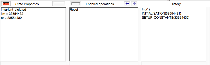

Symbolic Model Checking
Overview
The current nightly builds of ProB support different symbolic model checking algorithms:
- Bounded Model Checking (BMC),
- k-Induction, and
- different Variants of the IC3 algorithm.
As opposed to constraint-based checking, these algorithms find counterexamples which are reachable from the INITIALISATION. As opposed to ordinary model checking, they do not build up the state space explicitly, e.g., they do not compute all possible solutions for parameters and constants. This can be useful when the out-degree of the state-space is very high, i.e., when there are many possible solutions for the constants, the initialisation and/or the individual operations and their parameters.
In addition to the algorithms explained here, BMC*, a bounded model checking algorithm based on a different technique is available in Prob. See its wiki page for details.
Usage
Take the following example:
MACHINE VerySimpleCounterWrong
CONSTANTS lim
PROPERTIES lim = 2**25
VARIABLES ct
INVARIANT
 ct:INTEGER & ct < lim
INITIALISATION ct::0..(lim-1)
OPERATIONS
  Inc(i) = PRE i:1..1000 & ct + i <= lim THEN ct := ct+i END;
  Reset = PRE ct = lim THEN ct := 0 END
END
The ProB model checker will here run for a very long time before uncovering the error that occurs when ct is set to lim. If you run the TLC backend you will get the error message "Too many possible next states for the last state in the trace."
However, for the symbolic model checking techniques this is less of a problem. You can use them via command-line version of ProB as follows:
$ probcli VerySimpleCounterWrong.mch -symbolic_model_check bmc
K = 0
solve/2: result of prob: contradiction_found
K = 1
solve/2: result of prob: contradiction_found
K = 2
solve/2: result of prob: contradiction_found
K = 3
solve/2: result of prob: contradiction_found
K = 4
solve/2: result of prob: solution
successor_found(0)
 --> INITIALISATION(0)
successor_found(1)
 --> Inc
successor_found(2)
 --> Inc
successor_found(3)
 --> Inc
successor_found(4)
 --> Inc
! *** error occurred ***
! invariant_violation
Instead of "bmc" you can use "kinduction" and "ic3" as command line arguments in order to use the other algorithms.
The algorithms are also available from within ProB Tcl/Tk. They can be found inside the "Symbolic Model Checking" sub-menu of the "Analyse" menu.
More details
A paper describing the symbolic model checking algorithms and how they are applied to B and Event-B machines has been submitted to ABZ 2016.
Refinement Checking
| Warning This page has not yet been reviewed. Parts of it may no longer be up to date |
ProB can be used for refinement checking of B, Z and CSP specifications. Below we first discuss refinement checking for B machines. There is a tutorial on checking CSP assertions in ProB which can be viewed here.
What kind of refinement is checked?
ProB checks trace refinement. In other words, it checks whether every trace (consisting of executed operations with their parameter values and return values) of a refinement machine can also be performed by the abstract specification.
Hence, ProB does *not* check the gluing invariant. Also, PRE-conditions are treated as SELECT and PRE-conditions of the abstract machine are *not* always propagated down to the refinement machine. Hence, refinement checking has to be used with care for classical B machines, but it is well suited for EventB-style machines.
How does it work?
- Open the abstract specification, explore its state space (e.g.,using an exhaustive temporal model check).
- Use the command "Save state for later refinement check" in the "Verify" menu.
- Open the refinement machine.
- You can now use the "Refinement Check..." command in the "Verify" menu.
Testing
Also see Tutorial Model-Based Testing.
State Space Coverage Analyses
ProB provides various ways to analyse the coverage of the state space of a model. In ProB Tcl/Tk these features reside in the Coverage submenu of the Analyse menu:

These coverage commands all operate on the state space of the B model, i.e., those states that ProB has visited via animation or model checking from the initial states. Note: if you perform constraint-based checks, ProB may add additional states to this state space, which are not necessarily reachable from the initial states. Note: these commands do not drive the model checker and work on the currently explored state space; if the state space is incomplete the commands may obviously miss covered values in the unexplored part. Finally, the larger the state space, the more time these commands will take.
Here is a brief overview of the main commands:
- Operation Coverage: determine which operations (aka events for Event-B or actions for TLA) are covered in the state-space and compute how often each operation is enabled
- Minimum and Maximum Values: determine for each variable and constant a minumum and maximum value that is reached. This also detects whether just a single value was encountered. This command is particularly useful when model checking unexpectedly runs for very long or seems to run forever: here one can often spot individual variables which grow in an unbounded fashion.
- Value coverage for Expression: this allows the user to enter an expression, which is computed in every state of the state space; all values are then displayed in a table along with the possible values, how often these values have been encountered and a witness state id, giving you one possible witness state for this value.
- Number of covered values for variables: computes for each variable, how many different values it has taken on in the state space. Again, this is useful to diagnose state space explosion.
- Precise Operation Coverage: will check which operations have been covered in the current state space; for those operations that have not been covered, the constraint solver is called to determine whether the operation is actually feasible given the invariant (is there a state satisfying the invariant which enables the operation). If an operation is infeasible, it can never be reached (unless we reach a state violating the invariant).
The commands to determine vacuous guards and invariants rely on MC/DC coverage, which is detailed below.
MC/DC Coverage
MC/DC (Modified Condition/Decision Coverage) is a coverage criterion which is used in avionics. One core idea is ensure that for every condition in our code or model we generate at least one test where the condition independently plays an observable role in the outcome of a decision. In other words, if the condition were to be true rather than false (or vice versa) the decision would be changed. In still other words, we are trying to find an execution context where the result of the particular condition under test is crucial for the observable outcome.
In the context of B and Event-B, one question is what constitutes a condition and what constitutes a decision. We view a condition to be an atomic predicate (e.g., x>y) not involving logical connectives (&, or, not, =>, ⇔). There is, however, the possibility of treating a bigger predicate as atomic (e.g., an entire guard of an event). The reason for this is to provide better feedback to the user and to reduce the number of coverage criteria if desired. At the moment, we also consider a universally or existentially quantified formula to be a condition. A decision constitutes the fact whether an event is enabled or not. However, we also allow MC/DC to be applied in other contexts, e.g., to analyse invariants; in that setting a decision is whether an invariant is true or false.
We have implemented a MC/DC coverage analysis which examines all visited states and computes the MC/DC coverage for a series of predicates under consideration. Currently MC/DC coverage is used in two ways:
- for the coverage for the invariants, where the invariant is expected to be true (i.e., the analysis does not expect to find states where the invariant is false)
- for the coverage for the event guards. Here it is expected that every event can be enabled or disabled.
The algorithm is parametrised by an optional depth bound (called level in the coverage menu of ProB Tcl/Tk): if the depth bound is reached, then all sub-predicates are considered to be atomic decisions. The analysis can be used to measure the coverage of tests, but can also be used after an exhaustive model check to detect vacuous guards and vacuous invariants.
The MC/DC analysis has been integrated into ProB and has been successfully applied to various case studies. Below is a screenshot of part of the output for an early version of the ABZ landing gear case study. It shows that parts of the invariant inv13 not(C0step = 0 & (gearstate = retracting & doorstate /= locked_open & handle = UP)) cannot be set independently to false. This highlights a redundancy in the invariant; indeed the simpler to understand (but stronger) invariant not(gearstate = retracting & doorstate /= locked_open) holds.

Test Case Generation
Introduction
Testing aims at finding errors in a system or program. A set of tests is also called a test suite. Test case generation is the process of generating test suites for a particular system. Model-based Testing (MBT) is a technique to generate test suites for a system from a model describing the system. One usually tries to generate test suite which satisfies a given coverage criterion, e.g., ensuring that parts of the model are exhaustively exercised. Indeed, exhaustive testing of the implemented system is usually infeasible (because it would require infinitely many or way too many test cases), but one would like to increase the likelihood that the selected test suite uncovers errors in the implemented system.
In our case we have that
- a model is a formal model written in B, Event-B or even TLA+ and Z
- a test-case is a sequence of operations (or events) along with parameter values for the operations and concrete values for the constants and initial values of the formal model. One can also specify that a valid test case must end in a given class of states (specified by a predicate on the formal model's state).
- the coverage criterion is currently restricted to operation/event coverage, i.e., trying to ensure that every operation/event of the model is exercised by at least one test case.
ProB has two main algorithms to find suites of test cases:
- model-checking based (invoked, e.g., using the mcm_tests command of probcli) and
- constraint-based (invoked, e.g., using the cbc_tests command of probcli; more details can be found below)
The former will run the model checker to generate the state space of the formal model, and will stop when the coverage criterion has been satisfied. The full state space of the model contains all possible initialisations of the machine, along with all possible values of the constants. The latter will use ProB's constraint solver to generate feasible sequences of events in a breadth-first fashion and will also stop when the coverage criterion has been satisfied. (You may want to examine the Tutorial_Model_Checking,_Proof_and_CBC in this context.) So what are the differences:
- the constraint-based approach will instantiate the constants and parameters of the operations as required by the target sequence. It will not examine every possible valuation for the constants and initial values of the machine, nor every possible value for the parameters of the operation.
- the constraint-based approach hence does not construct the full-state space (aka a graph), but rather constructs a tree of feasible execution paths. The constraint-based approach cannot detect cycles; even if the state space is finite it may run forever in case an operations cannot be covered (because it is infeasible).
Model-Checking-Based Test Case Generation
Model-checking-based test case generation will build the model's state space, starting from the initial states, until the coverage criterion is satisfied. ProB uses a "breadth-first" approach to search for the test cases.
How to run
We will use the following B Machine as an example, which is stored in a file called simplecounter.mch.
MACHINE SimpleCounter
DEFINITIONS MAX==4
VARIABLES count
INVARIANT
 count: 1..MAX
INITIALISATION count := 1
OPERATIONS
  Increase(y) = PRE y: 1..(MAX-count) THEN
     count := count+y
  END;
  Reset = BEGIN count := 1 END
END
To start the test case generation there are two alternatives: Using the tcl/tk-application or the command line.
From the command line
From the command line there are two commands to configure the test case generation:
-mcm_tests Depth MaxStates EndPredicate File
        generate test cases with maximum length Depth, exploring MaxStates
        states; the last state satisfies EndPredicate and the
        test cases are written to File

-mcm_cover Operation(s)
        Specify an operation or event that should be covered when generating
        test cases. Multiple operations/events can be specified by seperating
        them by comma or by using -mcm_cover several times.
When all requested operations are covered by test cases within maximum length Depth, the algorithm will still explore the complete state space up to that maximum distance Depth from the initialisation. It outputs all found traces that satisfy the given requirements. The algorithm stops when it either
- has covered all required operations/events with(/and?) the current search depth
- or has reached the maximum search depth or maximum number of states to explore.
Example: To generate test cases that cover the event Increase in the machine above, leading to a state where count = MAX-1 is true, the explored paths do not have a depth of more than 5 operations and not more than 2000 states are explored, we would specify this as follows, where we have a timeout of 2000 ms for each explored trace:
./probcli.sh simplecounter.mch -mcm_tests 5 2000 count=MAX-1 test_results.xml -mcm_cover Increase
The generated test cases are stored in a file called test_results.xml. You can provide the empty filename "" in which case no file is generated. Providing the same as `EndPredicate` will only lead to test cases of length 1.
As of version 1.6.0, the operation arguments are also written to the XML file. The preference INTERNAL_ARGUMENT_PREFIX can be used to provide a prefix for internal operation arguments; any argument/parameter whose name starts with that prefix is considered an internal parameter and not shown in the trace file. Also, as of version 1.6.0, the non-deterministic initialisations are shown in the XML trace file: all variables and constants where more than one possible initialisation exists are written into the trace file, as argument of an INITIALISATION event.
In the tcl/tk-application
In the tcl/tk-application the test case generation can be started by choosing Analyse > "Testing" > "model-checking-based test case generation...". In the appearing window one can set the same parameters as described for the command line.

After a short while you will see the following window:

You cannot look at the test cases in ProB. Instead you can open the file you just saved the results to, which looks like this:
<extended_test_suite>
  <test_case id="1" targets="[Increase]">
    <global>
      <step id="1" name="Increase">
      <value name="y">4</value>
    </step>
    </global>
  </test_case>
</extended_test_suite>
Constraint-based Test Case Generation
Constraint based test case generation allows to explore the state space for a machine and generate traces of operations that cover certain user defined operations and meet a given condition to end the search. (See also the bounded model checker of ProB which uses this technique to find invariant violations.)
When should one use the constraint-based test case generator:
- when one has a large number of possible values for the constants
- when one has a large number of possible values for the initial values
- when one has a large number of possible values for the parameters of the operations
- when the lengths of the individual test-cases remains relatively low; indeed, the complexity of the constraint solving increases with the length of the test-case and the number of candidate test cases also typically grow exponentially with the depth of the feasible execution paths.
Example: When Constraint-based Test Case Generation is better
Here is an example which illustrates when constraint-based test case generation is better.
MACHINE Wiki_Example1
CONSTANTS n PROPERTIES n:NATURAL1
VARIABLES x, y INVARIANT x: 0..n & y:0..n
INITIALISATION x :: 1..n || y := 0
OPERATIONS
  Sety(yy) = PRE yy:1..n THEN y:=yy END;
  BothOverflow = SELECT x=y & y> 255 THEN x,y := 0,0 END
END
The state space of this machine is infinite, as we have infinitely many possible values for n. For large values of n, we also have many possible initialisations for x and may possible parameter values for the Sety operation. This gives us an indication that the constraint-based test-case generation algorithm is better suited. Indeed, it will very quickly generate two test cases:
- SETUP_CONSTANTS(1) ; INITIALISATION(1,0) ; Sety(1)
- SETUP_CONSTANTS(256) ; INITIALISATION(256,0) ; Sety(256) ; BothOverflow
For the second test, the constraint solver was asked to find values for n, x, y, and the parameter yy so that the following sequence is feasible:
- SETUP_CONSTANTS(n) ; INITIALISATION(x,y) ; Sety(yy) ; BothOverflow
The first solution it found was n=256,x=256,y=0,yy=256. The whole test-case generation process takes less than a second. The generated tree can be visualised by ProB:

One can see that the only path of length 1 (not counting the INITIALISATION step) consists of the operation Set. The possible paths of length 2 are Set;BothOverflow and Set;Set. (The latter is grayed out as it does not provide a new test case.) Within ProB's state space the following states are generated by the test case generator. As one can see only the values n=1 and n=256 were generated, as driven by ProB's constraint solver:

Finding a trace such that BothOverflow is enabled using the model checker will take much more time. Indeed, first one has to set MAXINT to at least 256 so that the value n=256 will eventually be generated. Then one has to set MAX_INITIALISATIONS also to at least 256 so that this value will actually be inspected by the model checker. Finally one has to set MAX_OPERATIONS also to at least 256 to generate yy=256; leading to a (truncated) state space of at least 16,777,216 states. Below is the state space just for the values n=1 and n=2 (which contains no state where BothOverflow is enabled):

How to run
We will again use the machine simplecounter.mch. To start the test case generation there are three alternatives: Using the tcl/tk-application or using the command line by either providing all settings as command line arguments or in a test description file.
From the command line
From the command line there are six relevant settings to configure the test case generation:
-cbc_tests Depth EndPredicate File
        generate test cases by constraint solving with maximum
        length Depth, the last state satisfies EndPredicate
        and the test cases are written to File

-cbc_cover Operation
        when generating CBC test cases, Operation should be covered. Each
        operation to be covered needs to be specified separately.

-cbc_cover_match PartialOpName
        just like -cbc_cover but for all operations whose name contains "PartialOpName"

-cbc_cover_final
        specifies that the events specified above should only be used as final events in test-cases.
        This option can lead to a considerable reduction in running time of the algorithm.

-p CLPFD TRUE
        flag to enable the CLPFD constraint solver to search the state space, which is highly recommended.

-p TIME_OUT x
        time out in milliseconds to abort the exploration of each possible trace
Example: To generate test cases that cover the event Increase in the machine above, leading to a state where count = MAX-1 is true and the explored paths do not have a depth of more than 5 operations we would specify this as follows, where we use CLPFD and have a timeout of 2000 ms. for each explored trace:
./probcli.sh simplecounter.mch -cbc_tests 5 count=MAX-1 test_results.xml -cbc_cover Increase -p CLPFD true -p TIME_OUT 2000
The generated test cases are stored in a file called test_results.xml. Just as with model-checking-based test case generation you can provide the empty filename
''
, in which case no file is generated, and an empty EndPredicate that will only lead to test cases of length 1.
With a test description file
The configuration for the test case generation can also be provided as an XML file. The format is shown below:
<test-generation-description>
  <output-file>OUTPUT FILE NAME</output-file>
  <event-coverage>
    <event>EVENT 1</event>
    <event>EVENT 2</event>
  </event-coverage>
  <target>TARGET PREDICATE</target>
  <!-- the parameters section contains parameters that are very ProB-specific -->
  <parameters>
    <!-- the maximum depth is the maximum length of a trace of operations/event,
         the algorithm might stop earlier when all events are covered -->
    <maximum-depth>N</maximum-depth>
    <!-- any ProB preference can be set that is listed when calling "probcli -help -v" -->
    <!-- other probably interesting preferences are MININT, MAXINT and TIME_OUT -->
  </parameters>
</test-generation-description>
Example: For our example the description file would look as follows.
<test-generation-description>
  <output-file>test_results.xml</output-file>
  <event-coverage>
    <event>Increase</event>
  </event-coverage>
  <target>count = MAX - 1</target>
  <parameters>
    <maximum-depth>5</maximum-depth>
    <!-- Please note: TIME_OUT (in milliseconds) is not a global time out, it is per trace -->
    <preference name="CLPFD" value="true"/>
    <!-- Please note: TIME_OUT (in milliseconds) is not a global time out, it is per trace -->
    <preference name="TIME_OUT" value="2000"/>
  </parameters>
</test-generation-description>
Assuming the test description above is stored in file named simple_counter_test_description.xml, we start the test case generation with the following call.
./probcli.sh simplecounter.mch -test_description simple_counter_test_description.xml
In the tcl/tk-application
In the tcl/tk-application the test case generation can be started by choosing Analyse > Testing > constraint-based test case generation.... In the appearing window one can set the same parameters as described for the command line.

After a short while you will see the following window:

Clicking on View CBC Test Tree will open a window showing the test cases. In this case there is only one test case generated. After just one execution of Increase the EndPredicate count=MAX-1 is satisfied and all operations that we specified are covered, hence the test case's depth is 1.

All three execution variants lead to the same output in the file test_results.xml:
<extended_test_suite>
  <test_case>
    <initialisation>
      <value type="variable" name="count">1</value>
    </initialisation>
    <step name="Increase">
      <value name="y">4</value>
      <modified name="count">5</modified>
    </step>
  </test_case>
</extended_test_suite>
Another model, for which the given EndPredicate cannot be satisfied after one step, leads to the following test cases and tree structure of possible traces:
<extended_test_suite>
  <test_case>
    <initialisation>
      <value type="variable" name="counter">8</value>
    </initialisation>
    <step name="Double" />
    <step name="Double" />
    <step name="Double" />
  </test_case>
  <test_case>
    <initialisation>
      <value type="variable" name="counter">8</value>
    </initialisation>
    <step name="Double" />
    <step name="Double" />
    <step name="Double" />
    <step name="Double" />
    <step name="Halve" />
  </test_case>
</extended_test_suite>

References
Constraint-based test-case generation using enabling analysis:
- Aymerick Savary, Marc Frappier, Michael Leuschel. Model-Based Robustness Testing in Event-B Using Mutation. Proceedings SEFM'2015.
Enabling Analysis:
- Ivaylo Dobrikov, Michael Leuschel. Enabling Analysis for Event-B. Sci. Comput. Program. 158: 81-99. 2018.
Explicit test-case generation:
- Sebastian Wieczorek, Vitaly Kozyura, Andreas Roth, Michael Leuschel, Jens Bendisposto, Daniel Plagge, Ina Schieferdecker. Applying Model Checking to Generate Model-Based Integration Tests from Choreography Models. Proceedings FATES 2009, TestCom 2009.
Visualisation
Graphical Viewer
Introduction
ProB can generate a wide range of visualizations for your models, e.g.:
- the statespace of a model
- the value of a particular formula
- various reduced representation of the statespace of a model
- one particular state of a model represented as a graph
Firstly, ProB generates a textual representation of a graph in the "dot" format. This information is typically saved to a file which has the same name and path as your main model but has a ".dot" extension. It then uses GraphViz to render this file. For this, it can either make use of the "dot" program to generate a Postscript file (generating a file with the ".ps" extension), or it uses a Dot-Viewer (such as "dotty") to view the file directly.
Setting up the Graphical Viewer
- GraphViz: in order to make use of the graphical visualization features, you need to install a version of GraphViz suitable for your architecture. More details can be found in Installation.
- Then use the command "Graphical Viewer Preferences..." in the "Preferences" Menu:
Then set or check the following preferences:
- Path/Command for dot program
- Path/Command for dot viewer (e.g., dotty)
Note: you can use the "Pick" button to locate the dot program and the dot viewer.
In case you want to use the Postscript option, also make sure that you have a viewer for Postscript files installed, and set the preference "Path/Command for Postscript viewer".
- You can select which viewer to use by going to the "Graphical Viewer" sub-menu of the "Preferences" Menu:
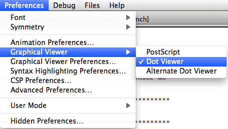 .
.

State Space Visualization
ProB provides several user-friendly visualization features to help the user to analyze and understand the behavior of his B specification. This feedback is very beneficial to the understanding of the B specification since human perception is good at identifying structural similarities and symmetries. For more information on this particular topic, the reader can refer to [1] and [2].
In this page we discuss the visualization of the state space of a specification. Visualizing individual states can be visualized using animation functions, Custom_Graph definitions or using VisB.
The visualization features of the state space are in the "Visualize" menu, and comprise the command (visualize) "Statespace" and all the commands of the sub-menu "Statespace Projections". It is important to understand that those commands operate on the state space computed by ProB at the current point during the animation. Each time the user animates the B specification, the state space computed by ProB can be expanded if the selected operations lead to states not already computed by ProB. As shown in the following figure, the command (visualize) "Statespace" displays a diagram corresponding to the state space currently explored by the animation in a separate window.

Graph Nodes
ProB displays the state space as a graph whose nodes correspond to states that are differentiated by their shapes and colors and arcs correspond to operations. The operations are all those that are displayed in the Enabled Operations pane except backtrack, which is only useful for animation. Four types of nodes are visualized in ProB:
- root The point before the B machine is initialized when it has no state;
- current The current state during the animation;
- normal The states that have been already computed during the animation;
- open The states that are reachable from the normal states by an enabled operation.
In addition to its type, a node can indicate that it corresponds to an invariant violation, which is displayed by a color filling as shown in the following figure

Finally, if you have specified a goal predicate (either using a DEFINITION GOAL == P or by using a command such as "Find state satisfying predicate...") then those predicates are coloured in orange. Many of the colours and shapes can be changed by adapting the corresponding preferences. A list of preferences is now shown automatically in ProB Tcl/Tk.
Statespace Projections
The sub-menu "Statespace Projections" contains several other commands that provide useful views on the state space.
- Transition Diagram for Custom Expression ...
- Signature-Merge Reduced Statespace...
- DFA Reduced Statespace
- Subgraph leading to Invariant Violation
- Subgraph for GOAL
Transition Diagram
The first command allows you to enter an expression (in B syntax). The command will then merge all states with the same value for that expression into an equivalence class node. In other words, the state space is projected onto the values of the expression. The generated graph contains only transitions which change the value of that expression (unless the DOT_LOOPS preference is set to true). The command allows one to project the state space onto a single variable, a subset of variables (by using a tuple (v1,v2,...,vk) as expression). You can increase the projection by using B operators such as card, ran, dom or any other B operator. A more detailed explanation is given in [2]. The command can also be called from probcli using these commands (in conjunction with other commands like --model-check):
probcli -dotexpr transition_diagram EXPR DOTFILE
The generated dot file can be viewed with a viewer like dotty or can be converted, e.g., to PDF using:
dot -Tpdf <DOTFILE >PDFFILE
Here is an example where a faulty lift model has been projected onto the expression
curfloor / 3

Signature and DFA Merge
The two next commands in the menu "View Visited States|View" provide a means to display a simplified version of the state space. A more detailed explanation is given in [1].
The command "Signature-Merge Reduced Statespace" displays a state space where nodes sharing the same output arcs are collapsed into one node. The command "Reducted Deterministic Automaton of Visited States" removes the non-determinacy of the state space graph. The command "Select Operations & Arguments for Reduction" is used to specify which operations and arguments are affected by the previous transformations.
Sub Graphs
The two last commands of the "Statespace Projections" sub-menu display subgraphs of the state space. The command "Subgraph for Invariant Violation" displays the subgraph of nodes which violate the invariant, while the command "Subgraph of nodes satisfying GOAL" displays the subgraph where goals (discussed in Temporal Model Checking) are satisfied.
As of December 2015, there is also a sub-menu "Statespace Fast Rendering", which enables one to visualize larger state spaces more effectively. Some sample visualizations can be found here.
Other Visualization Commands
The "Visualize" menu contains several other sub-menus, to visualize traces and individual states. The command "Shortest Trace to Current State" displays the shortest sequence of nodes in the state space starting from the root node and leading to the current node. The command "Current State" displays the current node and its successor nodes.
Preferences of the Visualization
Many aspects of the visualization can be configured in the "Graphical Viewer Preferences"... preference window of the "Preferences" menu. This includes changing the shapes and colors of the various nodes (using the notation of the dot tool, see Dot-Shapes and Dot-Colors). For selecting the colors, a color picker is available via the button Pick. The user can also select which labels to display on the nodes (value of variables) and arcs (operation arguments and return value of functions), and their font size.
The default graph viewer in ProB is dotty, which is from the Graphviz package. ProB enables the user to display the graph using a PostScript viewer by setting the preference Use PostScript Viewer in the Graphical Viewer Preferences to true.... The PostScript file is generated by the dot tool. The path to the PostScript viewer can be set in the "Path/Command" for PostScript Viewer preference. The "Pick" button can be used to select the path. WARNING: All paths to files and folders should use the / character to separate the folders and should be absolute.
Using a postscript viewer rather than dotty has several advantages and several drawbacks. Firstly, the assignment of node shapes and colors is more accurately realized by dot (and therefore PostScript). Dotty on the other hand is much easier to use when state spaces are large thanks to the birds-eye view. A PostScript viewer also has the advantage that the PostScript file may be used to capture visualizations for publication purposes.
At present, the distinction between using a PostScript viewer as opposed to dotty comes down to the difference in functionality between the !GraphViz utilities dot and dotty. The main differences with respect to visualization in ProB are are:
- For Postscript: Support for more visualization shapes (for example, the shape double-octagon appears as a box on dotty);
- Against PostScript: dot does not support the addition of shapes to arcs. With moderately large graphs, Dot may put nodes outside of the printable or viewable area. Examining large graphs in a PostScript viewer may be slow (it may be awkward to use pan and zoom). There is less support for information on arcs (for example, dotted lines).
- For Dotty: Graphs can be modified. Dotty includes a birds-eye viewer which is useful for examining large graphs.
- Against Dotty: Dotty may crash if the graph is too big or complex (and on Solaris and Linux if non-standard mouse buttons are used).
References
- ↑ 1.0 1.1 M. Leuschel and E.Turner: Visualising larger state spaces in ProB. In H. Treharne, S. King, M. Henson, and S. Schneider, editors, ZB 2005: Formal Specification and Development in Z and B, LNCS 3455. Springer-Verlag, 2005 https://www3.hhu.de/stups/downloads/pdf/LeTu05_8.pdf
- ↑ 2.0 2.1 L. Ladenberger and M. Leuschel: Mastering the Visualization of Larger State Spaces with Projection Diagrams. ICFEM'2015, LNCS 9407. Springer-Verlag, 2015. https://www3.hhu.de/stups/downloads/pdf/LadenbergerLeuschel_ProjectDiagram.pdf
State space visualization examples
(This page is under construction)
Alternating Bit Protocol
This is a visualisation of 3643 states and 11115 transitions of a TLA+ model of the alternating bit protocol, as distributed with the TLA+ tools. This model (MCAlternatingBit.tla) was loaded with ProB for TLA+, the model checker run for a few seconds and then the command "State Space Fast Rendering" with options (scale,fast) was used.
The goal predicate rBit=1 was used; those states satisfying this predicate are shown in orange.

Below is a projection of this state space onto the expression (rBit,sBit), using the "Custom Transition Diagram" feature of ProB:

More details about this statespace projection feature can be found in our ICFEM'15 article.
The main file of the model is:
--------------------------- MODULE MCAlternatingBit -------------------------
EXTENDS AlternatingBit, TLC

INSTANCE ABCorrectness

CONSTANTS msgQLen, ackQLen

SeqConstraint == /\ Len(msgQ) \leq msgQLen
                 /\ Len(ackQ) \leq ackQLen

SentLeadsToRcvd == \A d \in Data : (sent = d) /\ (sBit # sAck) ~> (rcvd = d)
=============================================================================

ImpliedAction == [ABCNext]_cvars

TNext == WF_msgQ(~ABTypeInv')
TProp == \A d \in Data : (sent = d) => [](sent = d)

CSpec == ABSpec /\ TNext

DataPerm == Permutations(Data)
==============================================================
MCInnerFIFO
This is a visualisation of 3866 states and 9661 transitions of a TLA+ model of a FIFO, as distributed with the TLA+ tools. This model (MCInnerFIFO) was loaded with ProB for TLA+ and the model checker run so that all states with queue size greater than qLen (3) were ignored, i.e., no successor states were computed (this can be set by defining SCOPE==card(q)<=qLen). The colour indicates the length of the queue variable q of the model (gray=0,blue=1,red=2, green=3, lightgray=4) .

Below is a projection of this state space onto the expression card(q), using the "Custom Transition Diagram" feature of ProB:

RushHour
This is a visualisation of the Rush_Hour_Puzzle Rush Hour puzzle B model, at the moment that ProB has found a solution to the goal predicate (red car moved out of the grid). The solution node(s) are marked in orange and the prism option was used.

Here is a visualisation of the full state space of 4782 nodes and 29890 transitions, using the scale option this time:

CAN Bus
This is a visualisation of the statespace of an Event-B model of a CAN Bus. The colours indicate the size of the BUSwrite variable (gray=0,blue=1,red=2, green=3, lightgray=4).

Hanoi (6 Discs)
This is a visualisation of the statespace of a B model of the towers of Hanoi for 6 discs. The state space contains 731 nodes and 2186 nodes.

One can observe that this figure resembles a Sierpinski triangle. This is no coincidence, the state space of Hanoi is one.
Below is a projection of this state space onto the expression card(on(dest))), using the "Custom Transition Diagram" feature of ProB:

Threads - Partial Order Reduction
This is the visualisation of a simple threads model, of two threads with n=51 steps before a synchronisation occurs and threads start again. The state space contains 5410 nodes. One can clearly see two synchronisation points on the left-hand side and right-hand side, and that in between synchronisation the processes simply interleave.

With partial order reduction, the state space is reduced to 208 states:

Here is the B source code of the model:
MACHINE Threads51
/* Two simple threads communicating from time to time
This kind of situation should happen quite often in controller systems
A partial-order reduction can hopefully reduce the interleavings
*/
DEFINITIONS
 ASSERT_LTL1 == "F deadlock(Step1_p1,Step1_p2)";
 HEURISTIC_FUNCTION == pc1 // for sfdp colouring
CONSTANTS n
PROPERTIES n = 51 /* n=51: 208 states with POR (deadlock checking), 5410 without */
VARIABLES pc1,pc2, v1,v2
INVARIANT
pc1 : NATURAL & pc2:NATURAL &
v1 :  INTEGER & v2:INTEGER
INITIALISATION pc1,pc2,v1,v2 := 0,0,0,0
OPERATIONS
 Step1_p1 = PRE pc1<n THEN /* maybe the fact that we have a decreasing variant has an influence on POR ? In Event-B this event would be convergent */
     pc1 := pc1+1|| v1 := v1+1
 END;
 Step1_p2 = PRE pc2<n /* & pc1=n manual POR */
             THEN /* also a convergent event (variant n-pc2) */
     pc2 := pc2+1 || v2 := v2+1
 END;
 Sync = PRE pc1=n & pc2=n THEN
    pc1, pc2 := 0,0 ||
    v1,v2 := v1 mod 2, v2 mod 2
 END
END
Below are projections of the above state spaces onto the expression (bool(pc1=n),bool(pc2=n)), using the "Custom Transition Diagram" feature of ProB.
The first shows the projection without partial order reduction:

With partial order reduction, one can see that the Step1_p1 events now all occur before the Step1_p2 events:

Eval Console
For this tutorial, load for example the file StackConstructive.mch included in the examples/Tutorial directory of the ProB distribution (this example is also discussed in the Tutorial Modeling Infinite Datatypes).
After loading the file, double click on the green line "SETUP_CONSTANTS" in the "Enabled Operations" pane. Now double click on the green "INITIALISATION" line in the same pane. To start the "Eval..." interactive console you can either
- use the "Eval..." command in the Analyse menu,
- double-click any line in the "State Properties" pane or
- right-click (Control-Click on a Mac) on the "State Properties" pane and select the "Eval..." entry as shown below:

This will bring up a new window, the "Eval Console":

You can now enter predicates or expressions and hit return or enter to evaluate them in the current state of the machine. Below is a small transcript:

You can use the up and down arrow keys to navigate to earlier predicates or expressions you have entered.
If you change the state, then the expressions and predicates are evaluated in that state. For example, if you execute the operations Push(RANGE3), Push(RANGE1), Push(RANGE2) by double-clicking on the respective lines in the "Enabled Operations" pane, then a transcript of using the console is as follows:

The console works the same way for Event-B models, Z and TLA specifications. However, in all those cases the Eval console uses the classical B parser and you have to use classical B syntax for entering predicates or expressions. The console also works in CSP mode and uses a CSP parser there.
As of version 1.4 the console allows defining new local variables (local to the console) using Haskell's let syntax: let id = Expr. You can use the :b command to browse your let definitions. Here is an example session:
>>> let x = 2**10
 1024
>>> let y = x+x
 2048
>>> :b
  x = 1024
  y = 2048
>>> {v| v>x & v<y & v mod x = 1}
 {1025}
>>>
A similar console is also available for the command-line version of ProB (probcli) using the -repl command. More details are available on the separate wiki page for probcli.
We now also have made two versions of a ProB Logic Calculator available online. The second one works similarly to the Eval console above, but is not linked to any B machine. You can try it out directly on this page below:
Evaluation View
This tutorial describes the use of ProB's evaluation view to explore single states of a model. The view shows the details of a particular state during the animation. It can be used to
- learn about the values of a some variables. This feature is overlapping with the State Properties View in the bottom left section of ProB's main window, but the evaluation view allows to inspect a value in greater detail.
- understand the truth value of the invariant and its sub-formulas and the values of the sub-expressions.
- export the content of variables in a state to use them outside of ProB.
Inspecting the State Variables and Constants
As an example specification we use the Sieve.mch delivered with the ProB Distribution in the "Less Simple" folder. After opening the model do a couple of animation steps and then open the Evaluation view in the Analyse menu. You should get window that looks similar to the following screenshot:

You can now expand each of the three sections to investigate the current state of the machine. For instance if we expand the Variables section we will get the following:

The tree shows values for each variable in the same way as the State Properties view. The value of the variable numbers in our example tell us that card(numbers) = 2288 and it shows the first and last entries. In contrast to the State Properties View you can see all values by doubleclicking an entry as shown in the next screenshot.

The save button can be used to save the value of the variable (as a B-Expression) to a file. You can also save the values of multiple variables (we will cover this later).
Understanding the Invariant and Properties
The second objective of the evaluation view is to help understanding why the invariant or the properties are true or false. Therefore the view allows us to expand a predicate into its sub-predicates and sub-expressions. This can be demonstrated using Priorityqueue.mch from the folder SchneiderBook. After initializing the machine and a few animation-steps opening the evaluation view yields

The invariant consists of two predicates
- queue : seq(NAT)
- !xx . (xx : 1..size(queue)-1 => (queue(xx) <= queue(xx+1)))
The first invariant is very simple. It is a predicate that has two sub-expressions queue and seq(NAT). The view shows the values for both subexpressions. Note that seq(NAT) is kept symbolic. The second invariant is more complex. It consistis of a sub-expression xx and and implication which has two sub-predicates xx : 1..size(queue)-1 and queue(xx) <= queue(xx+1)). As we see, the sub-predicates can also be expanded until we reach the level of simple values. The value of xx is chosen arbitrarily because the universal quantification is true. So let us modify the machine and introduce a bug e.g.
 insert(nn) =
 PRE nn : NAT
 THEN
   SELECT queue = <> THEN queue := [nn]
   WHEN queue /= <> & nn <= min(ran(queue)) THEN queue := queue <- nn /*<-- the bug */
   WHEN queue /= <> & nn >= max(ran(queue)) THEN queue := queue <- nn
   ELSE ANY xx
        WHERE xx : 1..size(queue)-1 & queue(xx) <= nn & nn <= queue(xx+1)
        THEN queue := (queue /|\ xx) ^ [nn] ^ (queue \|/ xx)
        END
   END
 END;
Now we can model check the machine and ProB will find a state that violates the invariant. Opening the evaluation view gives us something like

In the case that a universal quantification predicate yields false, ProB gives us a counterexample. For existential quantification the result is dual. If the predicate is true, we will get a witness, if it is false, we will get an arbitrarily chosen example.
In addition ProB has some built-in rules that allows us to better see, why a predicate has failed. For instance the predicate A <: B will contain a constructed sub-predicate B-A={}. If the original predicate is violated, then B - A it will contain precisely those elements that contradict the predicate. This makes it easy to spot the problem in particular if A and B are large sets. The behavior can be observed, for example, in the Paperround.mch model from the SchneiderBook folder. After a couple of operations the evaluation view looks like
If we introduce an error, such as
remove(hh) =
  PRE hh : 1..163
  THEN  papers := papers - {hh}
  END
we can now model check the machine and find a counter example that can be inspected using the evaluation view and because of the automatically introduced predicate it is very easy to see the reason why magazines <: papers is false.

Filtering relevant information and Data Extraction
There are two different ways to filter out important information from a state. To demonstrate this feature we can use the model SATLIB_blocksworld_medium.mch from the LessSimple folder of the ProB distribution. After executing SETUP_CONSTANTS and INITIALISATION we open the evaluation view. It contains a large number of constants and properties that might not be equally interesting.
The first way to filter out information is using the Search Box in the upper right part of the view. As we type, ProB will filter out all items that do not contain our search phrase. If we, for instance, type x19. We will get only those constants and properties that contain x19.

The second way to filter out unnecessary information is to mark some items and restrict the view. Suppose we are only interested in the constants x1, x4, x17 and the property (x4 = FALSE or X2=FALSE) or X6=TRUE (the first property in the list). Using the right mouse button, we can mark all the rows in the view that we want to see by selecting "Mark all selected items" from the context menu. In the same popup menu, we can select "Show only marked items" which will remove all other information.

Finally the popup menu allows us to save the content of a particular state into a file (either the full state, or the marked items only). In either case, ProB will generate a text file containing the state as a predicate. In our example the file will contain the following predicate
x1 = FALSE
 &
x4 = TRUE
 &
x17 = TRUE
 &
(x4 = FALSE or x2 = FALSE) or x6 = TRUE
Graphical Visualization
The graphical visualization of ProB [1] enables the user to easily write custom graphical state representations in order to provide a better understanding of a model. With this method, one assembles a series of pictures and writes an animation function in B. Each picture can be associated to a specific state of a B variable or expression. Then, depending on the current state of the model, the animation function in B stipulates which pictures should be displayed where. We now show how this animation can be done with very little effort.
As an alternative you can also specify CUSTOM_GRAPH definitions to render the current state as graph laid out by GraphViz. In addition, ProB also supports more powerful visualizations based on SVG and HTML in the form of VisB.
The Graphical Animation Model
The animation model is very simple. It is based on individual images and a user-defined animation function, which are both defined in the DEFINITIONS section of the animated machine as follows:
1. Each image is given a number and its source file location by using the following definition:
ANIMATION_IMGx == "filename", where x is the number of the image and "filename" is its path to a gif image file.
2. A user-defined animation function fa is evaluated to recompute the graphical output for every state. The graphical output of fa is known as the graphical visualization, which consists of a two-dimensional grid. Each cell in the grid can contain an image. The function uses the variables r (for row) and c (for column) to determine in which cell the image will be displayed. An image can appear multiple times in the grid.
The function fa is declared by defining ANIMATION_FUNCTION and ideally should be of type INTEGER * INTEGER +-> INTEGER. If the function fa is defined for r and c, then the animator should display the image with number fa(r,c) at row r and column c. If the function is undefined at this position, no image is displayed in the corresponding cell.
Notes: ProB will try and convert your expression to INTEGER * INTEGER +-> INTEGER (see below). Instead of an ANIMATION_IMGx one can also declare ANIMATION_STRx definitions for textual representations. If there is no image or string definition for the number fa(r,c) or if fa(r,c) is no number then ProB will try and display the result in pretty-printed textual format.
The dimension of the grid is computed by examining the minimum and maximum coordinates that occur in the animation function. More precisely,
the rows are in the range min(dom(dom(fa)))..max(dom(dom(fa))) and
the columns are in the range min(ran(dom(fa)))..max(ran(dom(fa))).
We take the B machine of the sliding 8-puzzle as an example. In the 8-puzzle, the tiles are numbered. Every tile can be moved horizontally and vertically into an empty square. The final configuration is reached whenever all the tiles are in order.
The B machine of the 8-puzzle is as follows:
MACHINE Puzzle8
DEFINITIONS INV == (board: ((1..dim)*(1..dim)) -->> 0..nmax);
GOAL == !(i,j).(i:1..dim & j:1..dim => board(i|->j) = j-1+(i-1)*dim);
CONSTANTS dim, nmax
PROPERTIES dim:NATURAL1 & dim=3 & nmax:NATURAL1 & nmax = dim*dim-1
VARIABLES board
INVARIANT INV
INITIALISATION board : (INV & GOAL)
OPERATIONS
 MoveDown(i,j,x) = PRE i:2..dim & j:1..dim &
                       board(i|->j) = 0 & x:1..nmax & board(i-1|->j) = x
                   THEN board := board <+ {(i|->j)|->x, (i-1|->j)|->0}
                   END;
 MoveUp(i,j,x) = PRE i:1..dim-1 & j:1..dim &
                          board(i|->j) = 0 & x:1..nmax & board(i+1|->j) = x
                 THEN board := board <+ {(i|->j)|->x, (i+1|->j)|->0}
                 END;
 MoveRight(i,j,x) = PRE i:1..dim & j:2..dim &
                        board(i|->j) = 0 & x:1..nmax & board(i|->j-1) = x
                    THEN board := board <+ {(i|->j)|->x, (i|->j-1)|->0}
                    END;
 MoveLeft(i,j,x) = PRE i:1..dim & j:1..dim-1 &
                       board(i|->j) = 0 & x:1..nmax & board(i|->j+1) = x
                   THEN board := board <+ {(i|->j)|->x, (i|->j+1)|->0}
                   END
END
On the left side of the following Figure, the non-graphical visualization is generated by ProB. It is readable, but the graphical visualization at the right side is much easier to understand.

The graphical visualisation is achieved with very little effort by writing in the DEFINITIONS section, the following animation function, as well as the image declaration list:
ANIMATION_FUNCTION == ( {r,c,i|r:1..dim & c:1..dim & i=0} <+ board);
ANIMATION_IMG0 == "images/sm_empty_box.gif"; /* empty square */
ANIMATION_IMG1 == "images/sm_1.gif"; /* square with 1 inside */
ANIMATION_IMG2 == "images/sm_2.gif";
ANIMATION_IMG3 == "images/sm_3.gif";
ANIMATION_IMG4 == "images/sm_4.gif";
ANIMATION_IMG5 == "images/sm_5.gif";
ANIMATION_IMG6 == "images/sm_6.gif";
ANIMATION_IMG7 == "images/sm_7.gif";
ANIMATION_IMG8 == "images/sm_8.gif"; /* square with lightblue 8 inside */
Each of the three integer types in the signature can be replaced by a deferred or enumerated set, in which case our tool translates elements of this set into numbers. In the case of enumerated sets, the number is the position of the element in the definition of the set in the SETS clause. Deferred set elements are numbered internally by ProB, and this number is used. (Note however, that the whole animation function has to be of the same type; otherwise the animator will complain about a type error.) To avoid having to produce images for simple strings, one can use a declaration ANIMATION_STRx == "my string" to define image with number x to be automatically generated from the given string.
Typical patterns for the animation function are as follows:
- A useful way to obtain a function of the required signature is to write a set comprehension of the following form:
{row,col,img | row:1..NrRow & col:1..NrCols & P},
 where P is a predicate which gives img a value depending on row and col.
- Another useful pattern is to write one function for default images and then use the override operator to replace the default images only when needed:
DefaultImages <+ CurrentImages
This was used in the 8-Puzzle by setting as default the empty square (image 0), which is then overriden by the partially defined board function.
- or to write multiple definitions of the animation function. More clearly, we define one animation function for default images and another one for current images as follows:
ANIMATION_FUNCTION_DEFAULT == DefaultImages;
ANIMATION_FUNCTION == CurrentImages;
Note: as of version 1.4 of ProB you can define multiple animation functions (e.g., ANIMATION_FUNCTION1, ANIMATION_FUNCTION2, ...) each overriding its predecessor.
This was used next in the Sudoku example.
- Translation Predicates between user sets and numbers (extension above can directly handle user sets but does not work well if we need a special image for undefined,...)
Further Examples
Below we illustrate how the graphical animation model easily provides interesting animations for different models.
Scheduler
The scheduler specification taken from [2] is as follows:
MACHINE scheduler
SETS PID = {process1,process2,process3}
VARIABLES active, ready, waiting
INVARIANT active <: PID & ready <: PID & waiting <: PID &
          (ready /\ waiting) = {} & active /\ (ready \/ waiting) = {} &
          card(active) <= 1 & ((active = {}) => (ready = {}))
INITIALISATION active := {} || ready := {} || waiting := {}
OPERATIONS
 new(pp) =
  SELECT pp : PID & pp /: active & pp /: (ready \/ waiting)
  THEN waiting := (waiting \/ { pp })
  END;
 del(pp) =
  SELECT pp : waiting
  THEN waiting := waiting - { pp }
  END;
 ready(rr) =
  SELECT rr : waiting
  THEN waiting := (waiting - {rr}) ||
       IF (active = {})
       THEN active := {rr}
       ELSE ready := ready \/ {rr}
       END
  END;
 swap =
  SELECT active /= {}
  THEN waiting := (waiting \/ active) ||
       IF (ready = {}) THEN active := {}
       ELSE
        ANY pp WHERE pp : ready
        THEN active := {pp} || ready := ready - {pp}
        END
       END
  END
END
The left side of the following Figure shows the non-graphical animation of the machine scheduler, and the right side shows its graphical animation obtained using ProB.

The graphical visualization is done by writing in the DEFINTIONS section the following animation function. Here, we need to map PID elements to image numbers.
IsPidNrci == p=process1 & i=1) or (p=process2 & i=2) or (p=process3 & i=3));
ANIMATION_FUNCTION ==
 ({1|->0|->5, 2|->0|->6, 3|->0|->7} \/ {r,c,img|r:1..3 & img=4 & c:1..3} <+
 ({r,c,i| r=1 & i:INTEGER & c=i & #p.(p:waiting & IsPidNrci)} \/
 {r,c,i| r=2 & i:INTEGER & c=i & #p.(p:ready & IsPidNrci)} \/
 {r,c,i| r=3 & i:INTEGER & c=i & #p.(p:active & IsPidNrci)} ));
ANIMATION_IMG1 == "images/1.gif";
ANIMATION_IMG2 == "images/2.gif";
ANIMATION_IMG3 == "images/3.gif";
ANIMATION_IMG4 == "images/empty_box.gif";
ANIMATION_IMG5 == "images/Waiting.gif";
ANIMATION_IMG6 == "images/Ready.gif";
ANIMATION_IMG7 == "images/Active.gif"
The previous animation function of scheduler can also be rewritten as follows:
ANIMATION_FUNCTION_DEFAULT ==
 ( {1|->0|->5, 2|->0|->6, 3|->0|->7} \/ {r,c,img|r:1..3 & img=4 & c:1..3} );
ANIMATION_FUNCTION == ({r,c,i| r=1 & i:PID & c=i & i:waiting} \/
                       {r,c,i| r=2 & i:PID & c=i & i:ready} \/
                       {r,c,i| r=3 & i:PID & c=i & i:active}
                      );
Sudoku
Using ProB we can also solve Sudoku puzzles. The machine has the variable Sudoku9 of type 1..fullsize-->(1..fullsize+->NRS), where NRS is an enumerate set {n1, n2, ...} of cardinality fullsize.
The animation function is as follows:
Nri == ((Sudoku9(r)(c)=n1 => i=1) & (Sudoku9(r)(c)=n2 => i=2) &
        (Sudoku9(r)(c)=n3 => i=3) & (Sudoku9(r)(c)=n4 => i=4) &
        (Sudoku9(r)(c)=n5 => i=5) & (Sudoku9(r)(c)=n6 => i=6) &
        (Sudoku9(r)(c)=n7 => i=7) & (Sudoku9(r)(c)=n8 => i=8) &
        (Sudoku9(r)(c)=n9 => i=9)
       );
ANIMATION_FUNCTION == ({r,c,i|r:1..fullsize & c:1..fullsize & i=0} <+
                       {r,c,i|r:1..fullsize & c:1..fullsize &
                       c:dom(Sudoku9(r)) & i:1.. fullsize & Nri}
                      );
The following Figure shows the non-graphical visualization of a particular puzzle (left), the graphical visualization of the puzzle (middle), as well as the visualization of the solution found by ProB after a couple of seconds (right).

Note that it would have been nice to be able to replace Nri inside the animation function simply by i = Sudoku9(r)(c). While our visualization algorithm can automatically convert set elements to numbers, the problem is that there is a type error in the override: the left-hand side is a function of type INTEGER*INTEGER+->INTEGER, while the right-hand side now becomes a function of type INTEGER*INTEGER+->NRS. One solution is to write multiple definitions of the animation function. In addition to the standard animation function, we can define a default background animation function. The standard animation function will override the default animation function, but the overriding is done within the graphical animator and not within a B formula. In this way, one can now rewrite the above animation as follows:
ANIMATION_FUNCTION_DEFAULT == ( {r,c,i|r:1..fullsize & c:1..fullsize & i=0} );
ANIMATION_FUNCTION == ({r,c,i|r:1..fullsize & c:1..fullsize &
                       c:dom(Sudoku9(r)) & i:1.. fullsize & i = Sudoku9(r)(c)}
                      )
Other Features
One can define actions for right clicks and mouse clicks and drags:
ANIMATION_RIGHT_CLICK(col,row) == SUBSTITUTION

ANIMATION_CLICK(fromcol,fromrow,tocol,torow) == SUBST
The allowed substitutions are currently limited:
- ANY, LET: to introduce wild cards; predicates will not (yet) be evaluated !!
- IF-ELSIF-ELSE: conditions have to be evaluable using the parameters only
- CHOICE: to provide multiple right click actions
One can set the font being used using ProB preferences. The following leads to a Monospaced font being used, making lining up of columns easier:
  SET_PREF_TK_CUSTOM_STATE_VIEW_FONT_NAME == "Monaco";
  SET_PREF_TK_CUSTOM_STATE_VIEW_FONT_SIZE == 9;
The following preferences can be used to control padding around cells:
  SET_PREF_TK_CUSTOM_STATE_VIEW_STRING_PADDING == Nr
  SET_PREF_TK_CUSTOM_STATE_VIEW_PADDING == Nr
The following preference can be used to disable the custom graphical visualization view:
SET_PREF_TK_CUSTOM_STATE_VIEW_VISIBLE == FALSE
One can control justification of animation strings using either of the two following DEFINITIONS:
ANIMATION_STR_JUSTIFY_LEFT == TRUE
ANIMATION_STR_JUSTIFY_RIGHT == TRUE
References
- ↑ M. Leuschel, M. Samia, J. Bendisposto and L. Luo: Easy Graphical Animation and Formula Viewing for Teaching B. In C. Attiogbé and H. Habrias, editors, Proceedings: The B Method: from Research to Teaching, pages 17-32, Nantes, France. APCB, 2008.
- ↑ B. Legeard, F. Peureux, and M. Utting. Automated boundary testing from Z and B. Proceedings of FME’02, LNCS 2391, pages 21–40. Springer-Verlag, 2002.
Command Line
ProB Cli
The ProB Cli (command-line interface) offers many of the ProB features via command-line. As such, you can run ProB from your shell scripts or in your Makefiles. probcli contains a REPL (Read-Eval-Print-Loop) and you can also integrate probcli into an editor such as vim. probcli can also communicate with other tools or graphical user interfaces via sockets (this is used by ProB for Rodin).
Documentation
Using the Command-Line Version of ProB
The command-line version of ProB, called probcli, offers many of the features of the standalone Tcl/Tk Version via the command-line. As such, you can run ProB from your shell scripts or in your Makefiles. These pages refer to version 1.6 of ProB. Some features are only available in the nightly build of ProB. You can run probcli –help to find out which commands are supported by your version of ProB. For Bash users we provide command completion support.
Note: the order of commands is not relevant for probcli (except within groups of commands such as -p MAXINT 127). Any argument that is not recognised by probcli is treated as a filename to be analysed.

Conventions used
The following conventions are used in this guide:
| <replaceme> | All values that should be replaced with some value are shown withing < > |
| line breaks | Command synopsis for command may be broken up on several lines. When typing commands enter all option on the same line. |
Synopsis
probcli [--help]
<filename> [ <options> ]
The underscore within all options can as of version 1.5.1-beta7 be replaced with dashes. Also, all commands can either be typed with single leading dashes or double leading dashes. For example, all of the following commands have the same effect:
probcli M.mch -model_check
probcli M.mch -model-check
probcli M.mch --model_check
probcli M.mch --model-check
Options
-mc <nr>
Description
| model check; checking at most <nr> states |
Example
probcli my.mch -mc 100
Note: with a value of nr=1 ProB will only inspect the "virtual" root node (and compute its outgoing transitions). Also see the related options -nodead, -noinv, -nogoal, -noass to influence which kinds of errors are reported by -mc. You can also set a target goal predicate using the -goal "PRED" command and limit the scope of the model checking using the -scope "PRED" command.
-model_check
The same as -mc but without a limit on the number of nodes checked. ProB will run until the entire state space is explored.
-no<x>
Description
restrict errors reported by model checking (-mc), TLC model checking (-mc_with_tlc), animation (-animate) and execution (-execute) with <x>=dead,inv,goal,ass
|
Example
probcli my.mch -mc 1000 -nodead -nogoal
-disable_timeout
Description
| turn off ProB's timeout mechanism, e.g., for computing enabled operations and invariant checking; this can sometimes speed up model checking (-mc or -model_check) and animation (-animate). Available as of version 1.5.1-beta7. |
Example
probcli my.mch -model-check -disable-timeout
-bf
Description
| proceed breadth-first during model checking |
Example
probcli my.mch -bf -mc 1000
-df
Description
| proceed depth-first during model checking |
Example
probcli my.mch -df -mc 1000
-mc_mode <M>
Description
influence how the model checker proceeds. Available as of version 1.5.1. Supersedes the -df and -bf switches.
Possible values for the mode <M> are:
|
Example
probcli my.mch -model_check -mc_mode random
--timeout <N>
Description
| Global timeout in ms for model checking and refinement checking.
This does not influence the timeout used for computing individual transitions/operations. This has to be set with the -p TIME_OUT <N>. Note that the TIME_OUT preference also influences other computations, such as invariant checking or static assertion checking, where it is multiplied by a factor. See the description of the -p option. |
Example
probcli my.mch -timeout 10000
-t
Description
| trace check (associated .trace file must exist) |
Example
probcli my.mch -t
-init
Description
| initialise specification |
Example
probcli my.mch -init
nr_of_components(1)
% checking_component_properties(1,[])
% enumerating_constants_without_constraints([typedval(fd(_24428,ID),global(ID),iv)])
% grounding_wait_flags
grounding_component(1)
grounding_component(2)
% found_enumeration_of_constants(0,2)
% backtrack(found_enumeration_of_constants(0,2))
% found_enumeration_of_constants(0,1)
% backtrack(found_enumeration_of_constants(0,1))
<- 0: SETUP_CONSTANTS :: root
% Could not set up constants with parameters from trace file.
% Will attempt any possible initialisation of constants.
 | 0: SETUP_CONSTANTS success -->0
 - <- 1: INITIALISATION :: 0
% Could not initialise with parameters from trace file.
% Will attempt any possible initialisation.
ALL OPERATIONS COVERED
 -  | 1: INITIALISATION success -->2
 -  - SUCCESS
-cbc <OPNAME>
Description
| constraint-based invariant checking for an operation (also use <OPNAME>=all) |
Example
probcli my.mch -cbc all
-cbc_deadlock
Description
| Perform constraint-based deadlock checking (also use -cbc_deadlock_pred PRED) |
This will try to find a state which satisfies the invariant and properties and where no operation/event is enabled. Note: if ProB finds a counter example then the machine cannot be proven to be deadlock free. However, the particular state may not be reachable from the initial state(s). If you want to find a reachable deadlock you have to use the model checker.
-cbc_deadlock_pred <PRED>
Description
| Constraint-based deadlock finding given a predicate |
This is like -cbc_deadlock but you provide an additional predicate. ProB will only find deadlocks which also make this predicate true.
Example
probcli my.mch -cbc_deadlock_pred "n=15"
-cbc_assertions
Description
| Constraint-based checking of assertions on constants |
This will try and find a solution for the constants which make an assertion (on constants) false.
You can use the extra command -cbc_output_file FILE to write the result of this check to a file. You can also use the extra command -cbc_option contradiction_check to ask ProB to check if there is a contradiction in the properties (in case the check did not find a counter-example to the assertions). The extra command -cbc_option unsat_core tells ProB to compute the unsatisfiable core in case a proof the assertions was found. Note that the TIME_OUT preference is multiplied by 10 for this command.
There are various variations of this command:
-cbc_assertions_proof
-cbc_assertions_tautology_proof
Both commands do not allow enumeration warnings to occur. The latter command ignores the PROPERTIES and tries to check whether the ASSERTION(s) are tautologies. Both commands can be useful to use ProB as a Prover/Disprover (as is done in Atelier-B 4.3).
-cbc_sequence <SEQ>
Description
| Constraint-based searching for a sequence of operation names (separated by semicolons) |
This will try and find a solution for the constants, initial variable values and parameters which make execution of the given sequence of operations possible.
Example
probcli my.mch -cbc_sequence "op1;op2"
-strict
Description
| raise error and stop probcli if anything unexpected happens, e.g., if model checking finds a counter example or trace checking fails or any unexpected error happens |
Example
probcli my.mch -t -strict
-expcterr <ERR>
Description
| expect error to occur (<ERR>=cbc,mc,ltl,...)
Tell ProB that you expect a certain error to occur. Mainly useful for regression tests (in conjunction with the -strict option). |
Example
probcli examples/B/Benchmarks/CarlaTravelAgencyErr.mch -mc 1000 -expcterr invariant_violation -strict
-animate <Nr>
Description
| random animation (max Nr steps) |
Animates the machine randomly, maximally Nr of steps. It will stop if a deadlock is reached and report an error. You can also use the command -animate_all, which will only stop at a deadlock (and not report an error). Be careful: -animate_all could run forever.
Example
probcli my.mch -animate 100
-execute <Nr>
Description
| execution (max Nr steps) |
Executes the "first" enabled operation of a machine, maximally Nr of steps. It will stop if a deadlock is reached and report an error. You can also use the command -execute_all, which will only stop at a deadlock (and not report an error). Be careful: -execute_all could run forever.
In contrast to -animate, -execute will
- always choose the first enabled operation it finds and stop searching for further enabled operations in that state (-animate will compute all enabled operations up to the limit set by the MAX_OPERATIONS or MAX_INITIALISATIONS preference and then choose randomly); the order of operations in the B machine is thus important for -execute
- not store intermediate states in the state space; as such -execute is faster but after execution one only has access to the first state and the final state of execution
Example
probcli my.mch -execute 100
-det_check
Description
| check if animation steps are deterministic |
Checks if every step of the animation is deterministic (i.e., only one operation is possible, and it can only be executed in one possible way as far as parameters and result is concerned). Currently this option has only an effect for the -animate <Nr> and the -init commands.
Example
probcli my.mch -animate 100 -det_check
-det_constants
Description
| check if animation steps are deterministic |
Checks if the SETUP_CONSTANTS step is deterministic (i.e., only one way to set up the constants is possible). Currently this option has only an effect for the -animate <Nr> and the -init commands.
Example
probcli my.mch -init -det_constants
-his <FILE>
Description
| save animation history to a file |
Save the animation (or model checking) history to a text file. Operations are separated by semicolons. The output can be adapted using the -his_option command. With -his_option show_states the -his command will also write out all states to the file (in the form of comments before and after operations). With -his_option show_init only the initial state is written out. The -his command is executed after the -init, -animate, -t or -mc commands. See also the -sptxt command to only write the current values of variables and constants to a file.
Example
probcli -animate 5 -his history.txt supersimple.mch
Additionally we can have the initialised variables and constants:
probcli -animate 5 -his history.txt -his_option show_init supersimple.mch
And we can have in addition the values of the variables in between (and at the end):
probcli -animate 5 -his history.txt -his_option show_states supersimple.mch
With -his_option trace_file as only option, probcli will write the history in Prolog format, which can later be used by the -t command.
-i
Description
| interactive animation |
After performing the other commands, ProB stays in interactive mode and allows the user to manually animate the loaded specification.
Example
probcli my.mch -i
-repl
Description
| start interactive read-eval-print-loop |
Example
probcli my.mch -p CLPFD TRUE -repl
A list of commands can be obtained by typing :help (just help for versions 1.3.x of probcli). The interactive read-eval-print-loop can be exited using :q (just typing a return on a blank line for versions 1.3.x of probcli).. If in addition you want see a graphical representation of the solutions found you can use the following command and open the out.dot file using dotty or GraphViz:
probcli -repl -evaldot ~/out.dot
You can also use the -eval command to evaluate specific formulas or expressions:
probcli -eval "1+2"
For convenience, these formulas can also be put into a separate file:
probcli -eval_file MyFormula.txt
-c
Description
| print coverage statistics |
Example
probcli my.mch -mc 1000 -c
You can also use the longer name for the command:
probcli my.mch -mc 1000 --coverage
There is also a version which prints a shorter summary (and which is much faster for large state spaces):
probcli my.mch -mc 1000 --coverage_summary
-cc <Nr> <Nr>
Description
| print and check coverage statistics
Print coverage statistics and check that the given number of nodes and transitions have been computed. |
Example
probcli my.mch -mc 1000 -cc 10 25
-p <PREFERENCE> <VALUE>
Description
| Set <PREFERENCE> to <VALUE>. For more information about preferences please have a look at Preferences |
You can also use --pref instead of -p. Example
probcli my.mch -p TIME_OUT 8000 -p CLPFD TRUE -mc 10000
-pref_group <PREFGROUP> <SETTING>
Description
| set to the group of preferences <PREFGROUP> to a predefined setting <SETTING> |
Example
probcli my.mch -pref_group model_check unlimited
Available groups and settings are:
- PREFERENCE GROUP integer : SETTINGS [int32] : Values for MAXINT and MININT
- PREFERENCE GROUP time_out : SETTINGS [disable_time_out] : To disable TIME_OUT
- PREFERENCE GROUP model_check : SETTINGS [disable_max,unlimited] : Model Checking Limits
- PREFERENCE GROUP dot_colors : SETTINGS [classic,dreams,winter] : Colours for Dot graphs
-prefs <FILE>
Description
| Set preferences from preference file <FILE>. The file should be created by the Tcl/Tk version of ProB; this version automatically creates a file called ProB_Preferences.pl. For more information about preferences please have a look at Preferences |
Example
probcli my.mch -prefs ProB_Preferences.pl
-card <GS> <VAL>
Description
| set cardinality (scope in Alloy terminology) of a B deferred set. This overrides the default cardinality (which can be set using -p DEFAULT_SETSIZE <VAL>). |
Example
probcli my.mch -card PID 5
-goal <PRED>
Description
| set GOAL predicate for model checker |
Example
probcli my.mch -mc 10000000 -goal "n=18" -strict -expcterr goal_found
-scope <PRED>
Description
| set SCOPE predicate for model checker; states which do not satisfy the SCOPE predicate will be ignored (invariant will not be checked and no outgoing transitions will be computed) |
Example
probcli my.mch -mc 10000000 -scope "n<18"
-s <PORT>
Description
| start socket server on given port |
Example
probcli my.mch ...
-ss
Description
| start socket server on port 9000 |
Example
probcli my.mch ...
-sf
Description
| start socket server on some free port |
Example
probcli my.mch ...
-sptxt <FILE>
Description
| save constants and variables to a file |
Save the values of constants and variables to a text file in classical B syntax. The -sptxt command is executed after the -init, -animate, -t or -mc commands. The values are fully written out (some sets, e.g., infinite sets may be written out symbolically).
See also the -his command.
Example
probcli -animate 5 -sptxt state.txt supersimple.mch
This will write the values of all variables and constants to the file state.txt after animating the machine 5 steps.
-cache <DIRECTORY>
Description
| save constants (and in future also variables) to a file to avoid recomputation |
This commands saves the values of constants for the current B machine and puts those values into files in the specified directory. The command will also tell ProB to try and reuse constants saved for subsidiary machines (included using SEES for example) whenever possible. The purpose of the command is to avoid recomputing constants as much as possible, as this can be very time consuming. This also works for values of variables computed in the initialisation or even using operations. However, we do not support refinements at the moment.
Note: this command can also be used when starting up the ProB Tcl/Tk version.
-logxml <LogFile>
Description
| log activities and results of probcli in XML format in <LogFile> |
A schema declaration file (xsd) can be found at doc/logxml_xsd.xml in the ProB Prolog sources. The log file contains information about the various commands performed by probcli. It also contains version information, the parameters provided to probcli and details about the errors that occured.
Example
probcli my.mch -mc 1000 -logxml log.xml
-logxml_write_vars <PREFIX>
Description
| after processing other commands (such as -execute) write values of variables having prefix PREFIX in their name into the XML log file (if XML logging has been activated using the -logxml command) |
Example
probcli my.mch -execute 1000 -logxml log.xml -logxml_write_vars out
-l <LogFile>
Description
| log activities in <LogFile> using Prolog format |
Example
probcli my.mch -mc 1000 -l my.log
-ll
Description
| log activities in /tmp/prob_cli_debug.log |
Example
probcli my.mch -mc 1000 -ll
-lg <LogFile>
Description
| analyse <LogFile> using gnuplot |
Example
probcli my.mch ...
-pp <FILE>
Description
| pretty-print internal representation to <FILE> |
Example
probcli my.mch -pp my_pp.mch
-ppf <FILE>
Description
| pretty-print internal representation to <FILE>, force printing of all type infos |
Example
probcli my.mch -ppf my_ppf.mch
-v
Description
| set ProB into verbose mode |
Example
probcli my.mch -mc 1000 -v
-version
Description
| print version information |
There is also an alternate command called -svers which just prints the version number of ProB. Example
probcli -version
ProB Command Line Interface
  VERSION 1.3.4-rc1 (9556:9570M)
  $LastChangedDate: 2011-11-16 18:36:18 +0100 (Wed, 16 Nov 2011) $
  Prolog: SICStus 4.2.0 (x86_64-darwin-10.6.0): Mon Mar  7 20:03:36 CET 2011
  Application Path: /Users/leuschel/svn_root/NewProB
probcli -svers
VERSION 1.3.4-rc1 (9556:9570M)
You can use probcli -version -v to obtain more information about your version of probcli.
-check_java_version
Description
| check Java and B parser version information |
This command is available as of ProB version 1.5.1-beta5 or higher. It can be useful to check that your Java is correctly installed and that the ProB B parser can operate correctly
probcli -check_java_version
Result of checking Java version:
 Java is correctly installed and version 1.7.0_55-b13 is compatible with ProB requirements (>= 1.7).
 ProB B Java Parser available in version: 2016-02-25 15:27:18.55.
-assertions
Description
| check ASSERTIONS of your machine
If you provide the -t switch, the ASSERTIONS will be checked after executing your trace. Otherwise, they will be checked in an initial state. ProB will automatically initialize the machine if you have not provide the -init or -t switch. You can also use -main_assertions to check only the ASSERTIONS found in the main file. If your ASSERTIONS are all static (i.e., make no reference to variables), then ProB will remove all CONSTANTS and PROPERTIES from your machine which are not linked (directly or indirectly) to the ASSERTIONS. This optimization will only be made if you provide no other switch, such as -mc or -animate which may require the computation of the variables. |
Example
probcli my.mch -init -assertions
-property
Description
| virtually add predicate to PROPERTIES |
Example
probcli my.mch -property "PRED"
-properties
Description
| check PROPERTIES
Note: you should probably first initialise the machine (e.g., with -init). If the constants have not yet been set up, probcli will debug the properties. |
Example
probcli my.mch -init -properties
-dot_output <PATH>
Description
| define path for generation of dot files for false properties or assertions |
This option is applicable to -properties and -assertions. It will result in individual dot files being generated for every false or unknown property or assertion. Assertions are numbered A0,A1,... and properties P0,P1,... You can also force to generate dot files for all properties (i.e., also the true ones) using the -dot_all command-line flag.
Example
probcli my.mch -init -properties -dot_output somewhere/
This will generate files somewhere/my_P0_false.dot, somewhere/my_P1_false.dot, ...
-rc
Description
| runtime checking of types/pre-/post-conditions |
Example
probcli my.mch ...
-ltlfile <FILE>
Description
| check LTL formulas in file <FILE> |
Example
probcli my.mch ...
-ltlassertions
Description
| check LTL assertions (in DEFINITIONS) |
Example
probcli my.mch ...
-ltllimit <LIMIT>
Description
| explore at most <LIMIT> states when model-checking LTL |
Example
probcli my.mch ...
-save <FILE>
Description
| save state space for later refinement check |
Example
probcli my.mch ...
-refchk <FILE>
Description
| refinement check against previous saved state space |
Example
probcli my.mch ...
-mcm_tests <Depth> <MaxStates> <EndPredicate> <FILE>
Generate test cases for the given specification. Each test case consists of a sequence of operations resp. events (a so-called trace) that
- start in a state after an initialisation
- contain a requested operation/event
- end in a state where the <EndPredicate> is fulfilled
The user can specify what requested operations/events are with the option -mcm_cover.
ProB uses a "breadth-first" approach to search for test cases. When all requested operations/events are covered by test cases within maximum length M, the algorithm will explore the complete state space with that maximum distance M from the initialisation. It outputs all found traces that satisfy the requirements above.
The algorithm stops if either
- it has covered all required operations/events with the current search depth
- or it has reached the maximum search depth or maximum number of explored states.
The required parameters are:
- Depth
- The maximum length of traces that the algorithm searches for test until it stops without covering all required operations/events.
- MaxStates
- The maximum number of explored states until the algorithm stops without covering all required operations/events.
- EndPredicate
- A predicate in B syntax that the last state of a trace must fulfil. If you do not have any restrictions on that state, use a trivially true predicate like 1=1
- FILE
- The found test cases a written to the XML file <FILE>.
Example
probcli my.mch -mcm_tests 10 2000 "EndStateVar=TRUE" testcases.xml -mcm_cover op1,op2
generates test cases for the operations op1 and op2 of the specification my.mch. The maximum length of traces is 10, at most 2000 states are explored. Each test case ends in a state where the predicate EndStateVar=TRUE holds. The found test cases are written to a file testcases.xml.
As of version 1.6.0, the operation arguments are also written to the XML file. The preference INTERNAL_ARGUMENT_PREFIX can be used to provide a prefix for internal operation arguments; any argument/parameter whose name starts with that prefix is considered an internal parameter and not shown in the trace file. Also, as of version 1.6.0, the non-deterministic initialisations are shown in the XML trace file: all variables and constants where more than one possible initialisation exists are written into the trace file, as argument of an INITIALISATION event.
-mcm_cover <Operation(s)>
Specify an operation or event that should be covered when generating test cases with the -mcm_test option. Multiple operations/events can be specified by seperating them by comma or by using -mcm_cover several times.
See -mcm-tests for further details.
-spdot <FILE>
Description
| Write graph of the state space to a dot <FILE> |
Example
probcli my.mch -mc 100 -spdot my_statespace.dot
-cbc_tests <Depth> <EndPredicate> <File>
Generate test cases by constraint solving with maximum length Depth, the last state satisfies EndPredicate and the test cases are written to File. If the predicate is the empty string we assume truth. If the filename is the empty string no file is generated. See also the page on Test_Case_Generation.
-cbc_cover <Operation>
When generating CB test cases, Operation should be covered. The option can be given multiple times to specify several operations.
Alternatively, multiple operations can be separated by a comma. You can also use the option
-cbc_cover_match PartialName
to match all operations whose name contains PartialName. See also the page about Test_Case_Generation.
-test_description <File>
Read the options for constraint based test case generation from File.
-bmc <Depth>
| Run the bounded model checker until maximum trace depth <Depth> specified. Looks for invariant violations using the constraint-based test case generation algorithm. |
Example
probcli my.mch -bmc 20
-csp-guide <File>
Use the CSP File File to guide the B Machine ("CSP||B"). (This feature is included since version 1.3.5-beta7.)
Environment Variables
Set NO_COLOR environment variable to disable terminal colors. See https://no-color.org.
Preferences
You can use these preferences within the command:
-p <PREFERENCE> <VALUE>
| <PREFERENCE> | <VALUE> |
|---|---|
| MAXINT | nat ==> MaxInt, used for expressions such as xx::NAT (2147483647 for 4 byte ints) |
| MININT | neg ==> MinInt, used for expressions such as xx::INT (-2147483648 for 4 byte ints) |
| DEFAULT_SETSIZE | nat ==> Size of unspecified deferred sets in SETS section. Will be used if a set s is neither enumerated, has no no card(s)=nr predicate in the PROPERTIES and has no scope_s == Nr DEFINITION. |
| MAX_INITIALISATIONS | nat ==> Max Number of Initialisations and ways to setup constants computed |
| MAX_OPERATIONS | nat ==> Max Number of Enablings per Operation Computed |
| ANIMATE_SKIP_OPERATIONS | bool ==> Animate operations which are skip or PRE C THEN skip |
| COMPRESSION | bool ==> Use more aggressive COMPRESSION when storing states |
| EXPAND_CLOSURES_FOR_STATE | bool ==> Convert lazy form back into explicit form for Variables, Constants, Operation Arguments. ProB will sometimes try to keep certain sets symbolic. If this preference is TRUE then ProB will try to expand those sets for variables and constants after an operation has been executed. |
| SYMBOLIC | bool ==> Lazy expansion of lambdas and set comprehensions. By default ProB will keep certain sets symbolic (e.g., sets it knows are infinite). When this preference is set to TRUE then all set comprehensions and lambda abstractions will at first be kept symbolic and only expanded into explicit form if needed. |
| CLPFD | bool ==> Use CLP(FD) solver for B integers (restricts range to -2^28..2^28-1 on 32 bit computers). Setting this preference to TRUE should substantially improve ProB's ability to solve complicated predicates involving integers. However, it may cause CLP(FD) overflows in certain circumstances. |
| SMT | bool ==> Enable SMT-Mode (aggressive treatment of : and /: inside predicates). With this predicate set to TRUE ProB will be better at solving certain constraint solving tasks. It should be enabled when doing constraint-based invariant or deadlock checking. ProB Tcl/Tk will turn this preference on automatically for those checks. |
| STATIC_ORDERING | bool ==> Use static ordering to enumerate constants which occur in most PROPERTIES first |
| SYMMETRY_MODE | [off,flood,nauty,hash] ==> Symmetry Mode: off,flood,canon,nauty,hash |
| TIME_OUT | nat1 ==> Time out for computing enabled transitions (in ms, is multiplied by a factor for other computations) |
| PROOF_INFO | bool ==> Use Proof Information to restrict invariant checking to affected unproven clauses. Most useful in EventB for models exported from Rodin. |
| TRY_FIND_ABORT | bool ==> Try more aggressively to detect ill-defined expressions (e.g. applying function outside of domain), may slow down animator |
| NUMBER_OF_ANIMATED_ABSTRACTIONS | nat ==> How many levels of refined models are animated by default |
| ALLOW_INCOMPLETE_SETUP_CONSTANTS | bool ==> Allow ProB to proceed even if only part of the CONSTANTS have been found. |
| PARTITION_PROPERTIES | bool ==> Partition predicates (PROPERTIES) into components |
| USE_RECORD_CONSTRUCTION | bool ==> Records: Check if axioms/properties describe a record pattern |
| OPERATION_REUSE | bool ==> Try and reuse previously computed operation effects in B/Event-B |
| SHOW_EVENTB_ANY_VALUES | bool ==> Show top-level ANY variable values of B Operations without parameters as parameters |
| RANDOMISE_OPERATION_ORDER | bool ==> Randomise order of operations when computing successor states |
| EXPAND_FORALL_UPTO | nat ==> When analysing predicates: max. domain size for expansion of forall (use 0 to disable expansion) |
| MAX_DISPLAY_SET | int ==> Max size for pretty-printing sets (-1 means no limit) |
| CSP_STRIP_SOURCE_LOC | bool ==> Strip source location for CSP; will speed up model checking |
| WARN_WHEN_EXPANDING_INFINITE_CLOSURES | int ==> Warn when expanding infinite closures if MAXINT larger than: |
| TRACE_INFO | bool ==> Provide various tracing information on the terminal/console. |
| DOUBLE_EVALUATION | bool ==> Evaluate PREDICATES positively and negatively when analyzing assertions or properties |
| RECURSIVE | bool ==> Lazy expansion of *Recursive* set Comprehensions and lambdas |
| IGNORE_HASH_COLLISIONS | bool ==> Ignore Hash Collisions (if true not all states may be computed, visited states are not memorised !) |
| FORGET_STATE_SPACE | bool ==> Do not remember state space (mainly useful in conjunction with Ignore Hash Collisions) |
| NEGATED_INVARIANT_CHECKING | bool ==> Perform double evaluation (positive and negative) when checking invariants |
| CSE | bool ==> Perform common-sub-expression elimination |
| CSE_SUBST | bool ==> Perform common-sub-expression elimination also for B substitutions |
Example
probcli my.mch -p TIME_OUT 5000 -p CLPFD TRUE -p SYMMETRY_MODE hash -mc 1000
Some probcli examples
To load a file My.mch, setup the constants and initialize it do:
probcli -init My.mch
To load a file M.mch, setup the constants, initialize and then check all assertions with Atelier-B's default values for MININT and MAXINT and an increased timeout of 5 seconds do:
probcli -init -assertions -p MAXINT 2147483647 -p MININT -2147483647 -p TIME_OUT 5000 M.mch
To fully model check a specification M.mch while tryining to minimize memory consumption do:
probcli -model_check -p COMPRESSION TRUE M.mch
To model check a specification M.mch while trying to minimize memory consumption further by not storing processed stats and using symmetry reduction (and accepting hash collisions) do:
probcli -p COMPRESSION -p IGNORE_HASH_COLLISIONS TRUE -p FORGET_STATE_SPACE TRUE -p SYMMETRY_MODE hash -model_check M.mch
Command-line Arguments for ProB Tcl/Tk
Note that the stand-alone Tcl/Tk version also supports a limited form of command-line preferences:
- FILE (the name/path of the file to be loaded)
- -prefs PREF_FILE (to use a specific preferences file, rather than the default ProB_Preferences.pl in your home folder)
- -batch (to instruct ProB not to try to bring up windows, but to print information only to the terminal)
- -selfcheck (to run the standard unit tests)
- -t (to perform the Trace Check on the default trace file associated with the specification)
- -tcl TCL_Command (to run a particular pre-defined Tcl command)
- -mc (to perform model checking)
- -c (to compute the coverage)
- -ref (to perform the default trace refinment check)
However, the comand-line version of ProB, called probcli, provides more features. It also does not depend on Tcl/Tk and can therefore be run on systems without Tcl/Tk.
Feedback
Please help us to improve this documentation by providing feedback in our bug tracker, asking questions in our prob-users group or sending an email to Michael Leuschel.
Other Languages
Also see the following tutorials:
- Tutorial Rodin First Step
- Tutorial Rodin Parameters
- Tutorial Rodin Exporting
- Tutorial Symbolic Constants
- Tutorial Disprover
- Tutorial CSP First Step
Other languages
Since version 1.2.7 of ProB (July 2008) you can also open Promela files with ProB. This mode is still experimental but already very usable and provides source-level highlighting during animation. The main purpose is to debug and animate Promela specifications in a user-friendly way. We do not plan to compete in terms of model checking speed with Spin (Spin compiles Promela to C code, ProB uses a Prolog interpreter). To animate a Promela model, simply open the file with the .pml or .prom extension with the "File->Open..." command. You will have to choose "Other Formalisms" or "All Files" in the filter pop-up-menu to be able to select the file.
You can also use ProB to animate and model check other specification languages by writing your own Prolog interpreter. To do this you should create a Prolog file with the .P extension and which defines three predicates:
- trans/3: this predicate should compute for every state (second argument), the outgoing transitions (first argument), and the resulting new states (third argument)
- prop/2: this predicate should compute the properties for the states of your system
- start/1: this defines the initial states of your system
For example, the following defines a system with two states (a and b) and two transitions (lock and unlock):
start(a). trans(lock,a,b). trans(unlock,b,a). prop(X,X).
These Prolog files can be loaded with ProB's open command (be sure to use the .P extension and to either choose "All files" or "Other Formalisms" in the file filtering menu).
Another simple example for a very basic process algebra is as follows:
% start(PossibleInitialState)
start(choice(pref(a,stop),intl(pref(b,pref(c,stop)),pref(d,stop)))).

% trans(Event, StateBefore, StateAfter)
trans(A,pref(A,P),P). % action prefix
trans(A,intl(P,Q),intl(P2,Q)) :- trans(A,P,P2). % interleave
trans(A,intl(P,Q),intl(P,Q2)) :- trans(A,Q,Q2).
trans(A,par(P,Q),par(P2,Q2)) :- trans(A,P,P2), trans(A,Q,Q2). % parallel composition
trans(A,choice(P,Q),P2) :- trans(A,P,P2). % choice
trans(A,choice(P,Q),Q2) :- trans(A,Q,Q2).

% prop(State, PropertyOfState)
prop(pref(A,P),prefix).
prop(intl(P,Q),interleave).
prop(A,A).
If you have a working interpreter, you can also contact the ProB developers in order for your interpreter to be included in the standard ProB distribution (in the style of the CSP-M or Promela interpreters). With this you can add syntax highlighting, error highlighting in the source code, highlighting during animation, support for new LTL properties,...
Another, slightly more elaborate example, is the following interpreter for regular expressions:
/* A simple animator for regular expressions */

start('|'('.'('*'(a),b) ,  '.'('*'(b),a))).

trans(_,[],_) :- !,fail.
trans(X,X,[]) :- atomic(X),!.
trans(X,'|'(R1,R2),R) :-
 trans(X,R1,R) ; trans(X,R2,R).
trans(X,'.'(R1,B),R) :- trans(X,R1,R2),
 gen_concat(R2,B,R).
trans(X,'?'(R1),R) :-
 trans(X,R1,R) ; (X=epsilon,R=[]).
trans(epsilon,'*'(_R1),[]).
trans(X,'*'(R1),R) :-
 trans(X,R1,R2),
 gen_concat(R2,'*'(R1),R).
trans(X,'+'(R1),R) :-
 trans(X,R1,R2),
 gen_concat(R2,'*'(R1),R).

gen_concat(R1,R2,R) :-
 (R1=[] -> R = R2 ; R = '.'(R1,R2)).

prop(X,X).
Finally, a more complex example is an encoding of the Rush Hour puzzle which also includes a graphical visualisation (using the animation_function_result predicate recognised by ProB as of version 1.4.0-rc3).
Other recognised Prolog predicates
The following can be used to set up an animation image matrix with corresponding actions:
- animation_image(Nr,Path)
- animation_function_result(State,List) where List is a list of terms of the form ((Row,Col),Img) where Img is either a declared animation_image number or another Prolog term
- animation_image_right_click_transition(Row,Col,TransitionTemplate)
- animation_image_click_transition(FromRow,FromCol,ToRow,ToCol,ListOfTransitionTemplates,ImageNr)
ProB for Event-B
In addition to classical B (aka B for software development), ProB also supports Event-B and the Rodin platform. ProB can be installed as a plugin for Rodin. Once installed, one can export contexts and models as *.eventb files and use them within ProB Tcl/Tk and the command-line version probcli.
See the tutorial pages for more information about using ProB for Event-B:
- Starting ProB for Rodin and First Animation Steps
- Important Parameters of ProB for Rodin
- Exporting Rodin Models for ProB Classic
- Using the Symbolic Contants Plugin
- Using the ProB (Dis-)Prover
- Visualization of LTL Counter-examples in Rodin
- Rodin Proof Obligations and Relation to ProB
The Rodin handbook also contains material about ProB:
ProB for Rodin
Currently there are two versions of ProB available for Rodin.
ProB (1) for Rodin
The first one is based on the old Java API and supports Rodin 2.8 and Rodin 3.3. The update site comes built in into Rodin, see the tutorial on installing ProB for Rodin. Nightly releases of this versions are also available on the Download page.
ProB 2.0 for Rodin
The second, still experimental, one is based on the new ProB Java API (aka ProB 2.0). Because the UI components provided by the ProB Java API are based on web technologies, we were able create a simple plugin for the Rodin 3 tool that provides the user with all of the functionality of ProB within Rodin. The plugin uses views with embedded Eclipse SWT browsers to access the user interface components that are shipped with the ProB Java API library. Details about nightly releases of this versions is also available on the Download page.
Multi-Simulation for Rodin based on ProB
There is now also a Multi-Simulation Plug-in available for Rodin. It enables discrete/continuous co-simulation.
Other Plug-Ins for Rodin
Prover Evaluation
This Plug-in is available at the update site http://nightly.cobra.cs.uni-duesseldorf.de/rodin_provereval/ and is capable to evaluate a variety of provers or tactics on a selection of proof obligations.
Camille
We also develop the Camille text-editor for Rodin. The update site (https://www3.hhu.de/stups/rodin/camille/nightly/) is preconfigured within Rodin. More information can be found on the Camille site at event-b.org.
Event-B
ProB supports animation and model-checking for Event-B specifications.
Installation
To install the ProB plugin for Rodin, open the "Help" menu in Rodin and click "Install new software".
You see a drop-down list titled "Work with:" at the top of the install dialog. Choose the update site "ProB - ..." and click on "ProB for rodin2" in the field below. Click on the "Next" button at the button on the dialog and proceed with the installation as usual.
Alternativaly, one can use the Tcl/Tk version of ProB but Event-B models must be exported to an .eventb file first (see below).
Animation and Modelchecking
You can start animation of a model (machine or context) by right-clicking on the model in the Event-B explorer. Choose "Start Animation / Model Checking".
TODO: Here we should add more details about the ProB perspective and views.
Export for use with the Tcl/Tk version of ProB
You can export a model (machine or context) to an .eventb - file by right-clicking on the model in the Event-B explorer. You can find the corresponding menu item right below the animation item.
Such a .eventb file can be opened by the command line and Tcl/Tk version of ProB.
Theories
ProB has (limited) support for theories.
Currently supported are (examples refer to the theory project below):
- recursive datatypes (e.g. the List datatype)
- operators defined by direct definitions (e.g. operators in the BoolOps theory) or recursive definitions (e.g. operators in the List theory)
- special annotated operators (see below)
Axiomatically defined operators are not supported without additional annotations.
Tagging operators
ProB has some extra support for certain operators. ProB expects an annotation to an operator that provides the information that it should use a specific implementation for an operator. Such tags are given in a .ptm file (ProB Theory Mapping). The file must have the same name as the theory.
For each annotated operator, the file contains a line of the form
operator Name internal {Tag}
where Name is the name of the operator in the theory and Tag is a ProB internal name.
The use of these tags is usually for experts only. In the theory file below, some of the theories are annotated.
Currently are the following tags supported:
| Tag | Description | Expected type |
|---|---|---|
| closure1 | the transitive closure | POW(T**T) |
| SIGMA | the sum of a set | POW(T**INT) |
| PI | the product of a set | POW(T**INT) |
| mu | ||
| choose | ||
| mkinat(op1,op2) |
TODO: to be continued...
Download Theories
An example project with theories: media:theories2.zip
TODO: A description of the supported parts.
Event-B Theories
ProB has (limited) support for theories.
Currently supported are (examples refer to the theory project below):
- recursive datatypes (e.g. the List datatype)
- operators defined by direct definitions (e.g. operators in the BoolOps theory) or recursive definitions (e.g. operators in the List theory)
- special annotated operators like transitive closure (see below)
Axiomatically defined operators are not supported without additional annotations.
Download Theories
An example project with theories: media:theories2.zip
The project contains the following theories:
- SUMandPRODUCT
- Contains two operators SUM and PRODUCT which take a set of the type POW(T**INT) as argument (with T being a type variable) and return the sum (resp.) product of all element's integer value.
The operators are annotated such that ProB uses an extra implementation.
- Seq
- The theory of sequences provides operators for sequences that are defined by direct definitions, thus supported by ProB.
- Real (unsupported)
- A theory of real numbers, currently unsupported by ProB.
- Natural
- A theory of inductive naturals (defined by a constant zero and a successor function).
- The mkinat operator is annotated such that ProB uses an explicit implementation.
- List
- A theory of lists that are either empty or have a head and a tail
- FixPoint (not really supported)
- The theory is defined by direct definitions but they usually get so complex that ProB cannot cope with them.
- closure
- The operator for transitive closure is supported by ProB.
- The operator is annotated such that ProB uses the classical B implementation.
- Card (contains no operators or data types)
- Contains theorem about set cardinalities.
- BoolOps
- Operators on Booleans (e.g. AND, OR) are defined by direct definitions and as such supported by ProB.
- BinaryTree
- Binary Trees are supported by ProB.
Tagging operators
ProB has some extra support for certain operators. ProB expects an annotation to an operator that provides the information that it should use a specific implementation for an operator. Such tags are given in a .ptm file (ProB Theory Mapping). The file must have the same name as the theory.
For each annotated operator, the file contains a line of the form
operator Name internal {Tag}
where Name is the name of the operator in the theory and Tag is a ProB internal name.
Currently are the following tags supported (with T being an arbitrary type):
| Tag | Description | Expected type | Return type |
|---|---|---|---|
| closure1 | the transitive closure | POW(T**T) | POW(T**T) |
| SIGMA | the sum of a set | POW(T**INT) | INT |
| PI | the product of a set | POW(T**INT) | INT |
| mu | returns the element of a singleton set | POW(T) | T |
| choose | returns (deterministically) one element of a non-emtpy set | POW(T) | T |
| mkinat(zero,succ) | returns an inductive natural number where zero and succ are the two operators of a natural number datatype with zero having no args and succ having one arg (an inductive natural) | INT | Inductive Nat |
As of version 1.12 (mid-september 2022) ProB also transparently accepts POW(INT) as type for SIGMA and PI. It now also accepts many of its external functions as tag names, such as the the functions from LibraryStrings.def or LibraryReals.def. For example, here we map the operator plus to ProB's external function RADD for adding two reals:
operator "plus" internal {RADD}
If you set the preference AUTO_DETECT_THEORY_MAPPING to TRUE then ProB will work with several standard Rodin theories even without a .ptm file in the workspace.
As of version 1.13 (November 2023) ProB also accepts literals as well as formulas between dollars in the .ptm files. For example, here the operator Rone is defined by the literal 1.0 and the operator RRealPlus by an expression (a set comprehension of the positive reals annotated with the symbolic pragma):
operator "Rone" internal {1.0}
operator "RRealPlus" internal {$/*@symbolic*/ {x|x:REAL & x>= 0.0}$}
Error Messages
In case the .ptm file is missing, you will get an error message such as the following one:
Axiomatic defined operator "SUM" not recognized.
Examples
For reference, here are the contents of some of the .ptm files. In case of an error message, you can copy these files into your Theory Projects (e.g., using Drag & Drop) and then refresh (F5). After that animation with ProB should work.
- SUMandPRODUCT.ptm
operator "SUM" internal {SIGMA}
operator "PRODUCT" internal {PI}
- closure.ptm
operator "cls" internal {closure1}
- Natural.ptm
operator "mk_iNAT" internal {mkinat}
Here are the contents for a Reals theory by Guillaume Dupont:
operator "RReal" internal {REAL}
operator "Rone" internal {1.0}
operator "Rzero" internal {zero}
operator "Rtwo" internal {two}
operator "plus" internal {RADD}
operator "times" internal {RMUL}
operator "minus" internal {RSUB}
operator "lt" internal {RLT}
operator "leq" internal {RLEQ}
operator "gt" internal {RGT}
operator "geq" internal {RGEQ}
operator "uminus" internal {RSUB}
operator "inverse" internal {RINV}
operator "divide" internal {RDIV}
operator "abs" internal {RABS}
operator "sqrt" internal {RSQRT}
operator "Rmax" internal {RMAXIMUM}
operator "Rmin" internal {RMINIMUM}
operator "RRealPlus" internal {$/*@symbolic*/ {x|x:REAL & x>= 0.0}$}
operator "RRealMinus" internal {$/*@symbolic*/ {x|x:REAL & x<= 0.0}$}
operator "RRealStar" internal {$/*@symbolic*/ {x|x:REAL & x /= 0.0}$}
operator "RRealPlusStar" internal {$/*@symbolic*/ {x|x:REAL & x> 0.0}$}
operator "RRealMinusStar" internal {$/*@symbolic*/ {x|x:REAL & x< 0.0}$}
CSP-M
ProB supports machine readable CSP[1] as supported by FDR and ProBE. CSP files can be animated and model checked on their own simply by opening a file ending with ".csp".
You can also use a CSP file to guide a B machine by first opening the B machine and then using the "Open Special" sub-menu of the File menu:
- use CSP file: uses the CSP file to control the current B machine (see below)
- use default CSP file: trys to use a CSP with the same name as the current B machine to control it
Limitations of CSP-M Support
ProB now supports FDR and ProBE compatible CSP-M syntax, with the following outstanding issues
- currying and lambda expressions have only been partially tested
- extensions and productions are not yet supported (but {| |} is)
- the priority of rename compared to external choice is unfortunately different than in FDR; please use parentheses
- mixing of closure with other set operations (especially diff) is not yet fully supported
- input patterns can only contain variables, tuples, integers and constants (ch?(x,1) is ok, ch?(y+1,x) not). Also, for a record, all arguments must be provided (e.g., for datatype r.Val.Val you have to write r?x?y you cannot write r?xy). Finally, for the moment within "ch? x.y:Set" the ":Set" associates only with y; if you want to check that "x.y" is in Set you need to write: "ch?(x.y):Set.
- channel declarations can either use associative dot tuples or non-associative tuples but not yet both. Also, sets of tuples as channel types will not work the same way as in FDR. I.e., for channel a:LinkData you should not use LinkData = {0.0, 0.1, 1.0, 1.1} but rather nametype LinkData = {0,1}.{0,1}.
Also, in the first phase we have striven for compatibility and coverage. We still need to tune the animator and model checker for efficiency (there are few known bottlenecks which will be improved, especially with deeply nested CSP synchronization constructs).
Guiding B Machines with CSP
To use this feature of ProB: first open a B Machine, then select "Use CSP File to Guide B..." or "Use Default CSP File" in the "Open Special" submenu of the File menu (you must be in normal user mode to see it).
The CSP file should define a process called "MAIN". This process will be executed in parallel with the B machine. The synchronization between the B machine and the CSP specification is as follows:
- CSP events that have the same name as B Operations will synchronize with B; CSP events that have the same name as a B Variable or Constant can be used to inspect the current value of these, all other CSP events can happen independently of B. In CSP terms the CSP and B are composed as follows:
CSP [| {op1,...,opn} |] Bwhere op1,...,opn are the visible operations defined in the B machine. - CSP events do not need to provide all arguments of B operations:
add!1 -> will match add(1,1) or add(1,2) or ...
(supposing add has 2 parameters in B)
add -> will match add(1,2), add(2,1), ...
add!1!2 -> will only match add(1,2)
- B Output arguments are specified at the end
lookup!X!2 will match lookup(X) --> 2
Note however, that for non-deterministic operations you generally should only retrieve the output value using a ? and not match against it using a !. Otherwise, the non-determinism of the B operation will be treated as an external choice for the CSP. So, if lookup is non-deterministic then we should do lookup!X?Res -> Res=2 & Cont rather than lookup!X!2 -> Cont. - If you have a variable called vv, then you can use vv?VAL to get the value of vv. You can also use, for example, vv!X to check that the value is equal to X. If vv is a relation or function, then you can also use two values on the channel to check for particular tuples in the relation. For example, use vv!3?Y to check whether tuples (3,Y) are in the relation vv (there will be one possible synchronisation per such value).
- see the file "bookstore_guide.csp" in the provided Machines directory for an example.
For the syntax definition see CSP-M Syntax
Command Line option for guided CSP||B
From the command line, you can specify a CSP File that should be used to guide the B machine with
-csp-guide <Filename>
(This feature is included since version 1.3.5-beta7.)
References
CSP-M Syntax
Details of supported CSP-M syntax
Note: you can use the command "Summary of CSP syntax" in ProB's help menu to get an up-to-date list of the supported syntax, along with current limitations.
PROCESS DEFINITIONS
- `Process = ProcessExpression`
PROCESS EXPRESSIONS
- `STOP` deadlocking process
- `SKIP` terminating process
- `CHAOS(a)` a: set of channel expressions
- `ch->P` simple action prefix where ch is a channel name possibly followed by a sequence of outputs "!v" and input "?VAR", where v is a value expression and VAR a variable identifier
- `ch?x:v->P` action prefix with set of accepted values
- `P ; Q` sequential composition
- `P ||| Q` interleaving
- `P [] Q` external choice
- `P |~| Q` internal choice
- `P /\ Q` interrupt
- `p [> Q` untimed timeout
- `P [| a |] Q` parallel composition with synchronisation on set of channel expressions a
- `P [ a || a' ] Q` alphabetised parallel
- `P [ c<->c' ] Q` linked parallel
- `P \ a` hiding of channel expressions in c
- `P [[ c<-c' ]]` renaming of channels c into c'
- `if B then P else Q`
- `b & P` guard using a boolean expression b
- `[]x:v@P` replicated external choice (x: variable, v: set value expression)
- `|~|x:v@P` replicated internal choice (x: variable, v: set value expression)
- `|||x:v@P` replicated interleave (x: variable, v: set value expression)
- `;x:s@P` replicated sequential composition (s: sequence expression)
- `||x:v@[a']P` replicated alphabetised parallel
- `[| a |]x:s@P` replicated sharing
- `[c<->c']x:s@P` replicated linked parallel (sequence s must be non empty)
- `let f1=E1 ... fk=Ek within P`
BOOLEAN EXPRESSIONS
- `true`
- `false`
- `b1 and b2` (`b1 && b2` also accepted but not in CSP-M)
- `b1 or b2` (`b1 || b2` also accepted but not in CSP-M)
- `b1 <=> b2` equivalence
- `b1 => b2` implication
- `not b`
- `v==w` equality of values
- `v!=w` disequality of values
- `v<w,v>w` strict ordering
- `v<=w,v>=w` non-strict ordering (v=<w also accepted)
- `member(v,w)` set membership check
- `empty(a)` set emptiness check
- `null(s)` sequence emptiness check
- `elem(x,s)` sequence member check
VALUE EXPRESSIONS
- `v+w`, `v-w` addition and subtraction
- `v*w` multiplication
- `v/w` integer division
- `v % w` division remainder
- `bool(b)` convert a boolean expression into a boolean value
- `{v,w,...}` enumerated sets
- `{m..n}` closed range
- `{m..}` open range
- `union(v,w)` set union
- `inter(v,w)` set intersection
- `diff(v,w)` set difference
- `Union(A)` generalized union of a set of sets
- `Inter(A)` generalized intersection
- `card(a)` cardinality of a
- `{x1,...,xn | x<-a,b}`
- `Events` all channel expressions on all declared channels
- `{| ... |}` closure of set of channel expressions
- `Set(a)` all subsets of a
- `<>` empty sequence
- `<v,w,...>` explicit sequence
- `<m..n>` closed range sequence
- `<m..>` open range sequence
- `<....>^s` sequence concatenation (first or last arg has to be an explicit sequence for patterns)
- `#s`, `length(s)`
- `head(s)`
- `tail(s)`
- `concat(s)`
- `set(s)` convert sequence into set
COMMENTS
- `-- comment until end of line`
- `{- arbitrary comment -}`
PRAGMAS
- `transparent f` where f is a unary function which will then on be ignored by ProB
- `{-# assert_ltl "f" "comment" #-}` where f is an LTL-formula and comment is an arbitrary comment, which is optional
- `{-# assert_ctl "f" "comment" #-}` where f is a CTL-formula and comment is an arbitrary comment, which is optional
Checking CSP Assertions
As of version 1.3.4, ProB provides support for refinement checking and various other assertions (deadlock, divergence, determinism, and LTL/CTL assertions) of CSP-M specifications. In this tutorial we give a short overview of the ProB’s implementations and features for checking CSP assertions. In the Tcl/Tk interface of ProB, CSP assertions can be assembled and checked in the CSP Assertions Viewer. A description of the CSP Assertions Viewer is also given.
Supported CSP Assertions in ProB
ProB provides support for checking almost all types of CSP-M assertions that can be checked within FDR2. Besides the assertion types that can be checked in FDR2, in ProB one also can check temporal properties on processes expressed by means of LTL and CTL formulae.[1] The following types of assertions are supported in ProB:
Refinement
Refinement is one of the fundamental notions for construction and verification of systems specified in CSP. Given two CSP processes P and Q one can state in ProB the property that process Q is an ‘m’ refinement of P by the following assertion declaration:
assert P [m= Q
where ‘m’ indicates one of the following types of comparison: ‘T’ for traces, ‘F’ for failures, ‘FD’ for failures-divergence, ‘R’ for refusals, and ‘RD’ for ‘refusals-divergence’. Note that the refinement types ‘V’ (revivals) and ‘VD’ (revivals-divergence) that are part of the refinement assertions supported by FDR2 are yet not supported by ProB.
Deadlock
Stating assertions about CSP processes to be deadlock-free is possible by the following assertion declaration:
assert P :[deadlock free [m]]
where P is a process expression and ‘m’ indicates one of the following models: ‘F’ (failures) and ‘FD’ (failures-divergence).
Determinism
Stating assertions about CSP processes to be deterministic is possible by the following assertion declaration:
assert P :[deterministic [m]]
where P is a process expression and ‘m’ one of the following models: ‘F’ (failures) and ‘FD’ (failures-divergence).
Livelock
Stating assertions about CSP processes to be livelock-free is possible by the following assertion declaration:
assert P :[livelock free]
where P is a process expression.
Temporal Properties
In ProB it is also possible to make assertions about temporal properties of CSP processes both in LTL and CTL. Basically, one wants to check whether some process P satisfies a formula f expressed in a temporal logic (denoted by P |= f).
To check whether a process P satisfies an LTL formula f write the following declaration:
assert P |= LTL: “f”
Note that f must be placed between quotes and that the satisfaction relation |= is immediately followed by `LTL:`. ProB supports LTL[e], an extended version of LTL which provides additionally support for making propositions on transitions. The following LTL[e] syntax for CSP-M specifications can be outlined by the following rules:
- Atomic propositions:
- To check if an event `evt` is enabled in a state use `e(evt)`
- Transition propositions:
- To check whether an event `evt` is executed use `[evt]`
- Logical operators
- `true` and `false`
- `not`: negation
- `&`,`or` and `=>`: conjunction, disjunction and implication
- Temporal operators:
- `G f`: globally
- `F f`: finally
- `X f`: next
- `f U g`: until
- `f W g`: weak-until
- `f R g`: release
- Fairness operators:
- `WF(evt)` or `wf(evt)`: weak fairness, where `evt` is an event
- `SF(evt)` or `sf(evt)`: strong fairness, where `evt` is an event
- `WEF` and `SEF` for checking LTL[e] formulae on executions that are strongly and weakly fair with respect to all events, respectively
An LTL[e] formula f is satisfied by some CSP process P if all executions of P satisfy f. If there is an execution of P which violates the property f, then the test P |= f fails by providing a counterexample. Depending on whether f expresses, a safety or liveness property, a finite path or a path in a lasso-form (, i.e. a path leading to a cycle) is returned as a counterexample, respectively.
Note that ProB supports also Past-LTL[e]. Past-LTL[e], however, may be considered to be inappropriate for LTL assertions since the goal of this type of assertions is usually to check whether all executions starting at the initial states of the process satisfy the respective LTL[e] formula.
To check whether a process P satisfies a CTL formula f the following assertion should be made:
assert P |= CTL: “f”
As for LTL, CTL formulae should be put in between quotes. The CTL syntax for CSP-M specifications could be summarised as follows:
- Atomic propositions:
- To check if an event `evt` is enabled in a state use `e(evt)`
- Transition propositions:
- To check whether an event `evt` is executed use `[evt]`
- State formulae, where f, f1 and f2 are path formulae:
- true | false | `not` f | f1 `&` f2 | f1 `or` f2 | f1 `=>` f2,
- E f : path quantifier ``, pronounced `for some path`
- A f : path quantifier ``, pronounced `for all paths`
- Path formulae, where g, g1 and g2 are state formulae:
- `X g`: next
- `g1 U g2`: until
- `G g`: globally
- `F g`: finally
- Next executed event:
- `EX [e] true`:


Note that these two types of assertions, the LTL and CTL assertions, are not part of the CSP-M language supported by FDR2. Loading a CSP-M file in FDR2 having assertion declarations of this form will exit with a syntax error. Bear in mind to remove or comment out such LTL/CTL assertions in the CSP-M file before loading it in FDR2.
CSP Assertions Viewer
When a CSP-M specification is loaded one can open the CSP Assertion Viewer either from the menu bar of the main window by selecting the `Check CSP-M Assertions` command in the `Verify` menu or from the Refinement button in the ‘’State Properties’’ pane. The viewer looks as follows:

The CSP Assertion Viewer of ProB has a similar design to the graphical user interface of FDR2. It consists basically of three main components: a menu bar, a list box and a tab pane. In the following each of the components and their corresponding functionalities are thoroughly described.
The Menu Bar
The menu bar is placed at the top of the window. On OS X, it is placed at the top of the screen. The menu bar includes several menus providing commands for adjusting, executing and changing the items in the list box, as well as some (standard) options for re-loading the model, saving the items to an external file or the loaded file, and launching some external tools related with the domain in which the list items are checked. Each menu can be popped up by a click with Mouse-1 (usually the left mouse button). The menu bar consists of the following menus and menu commands:
- File
- Reopen File: Reopening (re-reading and re-loading) the currently loaded file, incorporating any changes that may have been made since the file was last loaded.
- Copy new Assertions to File: All assertions that have been added to the list box since the currently loaded file was last read will be written to the file, i.e. all assertions that are yet not in the file are appended to it.
- Save Assertions to External File: Selecting the option opens a standard Tk dialog box requesting a name of a file in which the assertions and their results in the list box could be saved.
- Exit: Closing the CSP Assertion Viewer. Any assertion check results and any recently added assertions from the Tab Pane will get lost. The user will not be prompted to save these to the source file or an external file.
- Font
Changing the font settings of the elements in the list box. Each of the items of this menu is a cascading menu that provides a number of options to be selected. The currently selected option in the cascading menu is marked by a tick symbol (✓).- Family-Name: Change the font family of the text in the list box. There are currently four font families that could be chosen: Arial, Curier, Helvetica, and Times. Default font is Curier.
- Size: Change the font size of the text in the list box. Default font size is 10.
- Background: Change the background color of the list box. Default background color is Gray90.
- Assertions
The menu provides a list of commands for checking different types of assertions. In case a particular type of assertions is checked the respective command checks only these assertions that are not checked yet.- Uncheck All Assertions: Set the status of all assertions in the list box to non-checked (`?`).
- Delete All Assertions: Delete all assertions in the list box.
- Check All Refinement…: The item is a cascading menu and provides commands to check all assertions of one of the following supported refinement types: Traces, Failures, Failures-Divergence, Refusals, and Refusals-Divergence.
- Check Processes for…: The item is a cascading menu and provides commands to check all assertions of the following supported types of checks: Deadlock, Determinism and Livelock.
- Check All LTL Assertions: Selecting this command causes ProB to check all LTL assertions in the list box that are not checked yet.
- Check All CTL Assertions: Selecting this command causes ProB to check all CTL assertions in the list box that are not checked yet.
- Check All Assertions: Selecting this command causes ProB to check of all assertions in the list box that are not checked yet.
- External Tools
- Open Specification with FDR: Open the currently loaded CSP-M specification in FDR2. The FDR2 tool is launched with the currently loaded specification in case the FDR2 is installed and the correct path to the `fdr2` command is set for the respective preference `Path to the FDR2 tool`. The value of the `Path to the FDR2 tool` preference can be changed from the “CSP Preferences…” window which can be opened by selecting the `CSP Preferences…` command in `Preferences` menu of the main window.
- Evaluate with CSPM-Interpreter: Selecting this command opens a console in which one can evaluate CSP-M expressions using the CSP-M interpreter. The CSP-M interpreter is an external tool implemented independently from ProB. CSP-M expression can be evaluated if the `cspm` tool is installed and the path to the cspm-command is set for the respective preference `Path to CSPM tool`. The command is obsolete and its removal is considered in future.
The Assertion List Box
This part of the viewer lists all assertions stated in the currently loaded CSP-M specification and provides a set of features for checking, manipulating, and debugging of CSP assertions in the list. To each statement in the assertion list box a symbol is assigned, placed on the left side of it, that reveals the current status of the statement in the viewer:
- ? - Assertion not checked yet.
- ✔ - Assertion check completed successfully.
- ✘ - Assertion check completed, but a counterexample was found to the stated property. The debugger can be used to explore the reason why the property does not hold.
- ⌚ - Assertion is currently checked.
- ! - The check of the assertion not completed for some reason. Possible causes for the interruption may be:
- Syntax error in the property was detected;
- Assertion check failed because of missing implementation;
- Assertion check interrupted by user.
Note that in case of an LTL and a CTL assertion the check could fail to complete because of a syntax error in the respective formula. If an assertion check fails to complete an error box is popped up displaying an error message, which indicates why the assertion check could not be completed.
An assertion can be selected by clicking on it with Mouse-1 and checked by double-clicking on it with Mouse-1. Alternatively, selecting an assertion and then pressing the Enter key can start the respective assertion check. When an assertion check is in progress, the assertion will be marked by the clock symbol (⌚). If the assertion check is completed without interrupting it, a new status is assigned to the assertion: tick symbol (✔) indicating that the assertion was completed successfully or cross symbol (✘) indicating that a counterexample was found for the stated property. In case that the status is cross the counterexample can be explored by (second) double-click with Mouse-1 on the assertion or by selecting the assertion and then pressing the Enter key. If the respective assertion is negated, i.e. there is `not` in front of the assertion property, and marked with a cross, then no counterexample can be explored as the proper statement holds.
The list box is equipped with a contextual menu (or a pop-up menu), which appears when you right-click on an assertion in the list. Depending on the type and the status of the assertion the contextual menu provides options for checking, debugging, modifying the respective assertion, as well as various other options. Take, for example, the selected assertion on which the contextual menu is popped up in the picture below.

The assertion "ASSYSTEM |= LTL: “GF [eats.0]”" intends to check if the process ASSYSTEM satisfies the LTL formula "GF [eats.0]". For the selected assertion above, for example, the options `Show LTL Counterexample` and `Show LTL Counterexample in State Space` are enabled as a counterexample was found for the check. On the other hand, the options `Check Assertion` and `Interrupt Assertion` are disabled as the assertion check was completed.
The contextual menu has in general the following options:
The following options affect only the assertion being selected.
- Debug or Show LTL/CTL Counterexample…: Opens the graphical viewer for exploring the counterexample that was found for the respective LTL assertion check. Option is enabled if the assertion is not negated and its status is cross (✘), or if the assertion is negated and its status is tick (✔). Option appears if the assertion type is an LTL assertion or a CTL assertion.
- Debug Assertion: Opens a trace-failure debugger window showing the reason why the corresponding assertion check failed. Option is enabled if the assertion is not negated and its status is cross (✘), or if the assertion is negated and its status is tick (✔). Option available for all types of assertions except for LTL and CTL assertions.
- Check Assertion: Starts immediately the check of the assertion being selected before right clicking on it.
- Interrupt Assertion Check: Interrupts the current assertion check.
- Uncheck Assertion: If the assertion was checked and the result of the check is different from question mark (?), then the status of the assertion will be reset to question mark. Option is enabled only if the assertion result is different from question mark.
- Delete Assertion: Removes the selected item from the assertion list.
- Negate Assertion: Negates the respective assertion. If the result of the (proper) assertion check is cross (✘), then the result of the negated assertion becomes tick (✔). Otherwise, if the result of the (proper) assertion is tick (✔), the negated assertion becomes cross (✘).
- Swap Processes: Option available only for refinement assertions. Performing the command causes the attachment of a new refinement assertion in which the process expressions on both sides of the refinement operator `[m=` are swapped. If, for example, we execute ‘’Swap Processes’’ on the assertion "P [T= Q", the command adds to the list of assertions the assertion "Q [T= P".
The following options affect all assertions in the list box.
- Check All Assertions: The command causes the check of all assertions in the list box. The assertions that are already checked would not be checked again.
- Uncheck All Assertions: The status of all assertions in the list box is reset to question mark.
- Delete All Assertions: All entries in the list box are removed. As a result the message “No assertions were added.” appears in the list box.
Other options. The following options have no impact on the assertions in the list box.
- Summary of the CSP Syntax: Opens a window in which the summary of the CSP-M syntax and features supported by the ProB tool is given.
- Evaluate CSP Expressions: Opens the Eval console in which CSP expressions can be evaluated.
- Open Specification with FDR: Opens the currently loaded CSP-M specification in FDR2. The FDR2 tool is launched with the currently loaded specification if FDR2 is installed and the correct path to the `fdr2` command is set for the respective preference `Path to the FDR2 tool`. The value of the `Path to the FDR2 tool` preference can be changed from the “CSP Preferences…” window which can be opened by selecting the `CSP Preferences…` command in `Preferences` menu of the main window.
The Tab Pane
The tab pane is placed at the bottom of the window and enables the user to construct and check properties of processes of the currently loaded CSP-M file without adding explicitly assertions to the file.
There are overall six tab pages. Each tab page is used to build up new assertion statements. The tab pages provide selectors, entries and command buttons for assembling, adding and checking new assertions. In each of the selectors all possible processes of the loaded CSP-M file are accessible. It is also possible to specify new process expressions by entering these in the respective entry of the process selector. The tab pages for creating LTL and CTL assertions provide additionally an appropriate entry for specifying the according LTL and CTL formula intended to be checked on the specified process, respectively.
Each tab page is equipped with the following command buttons:
- Add: Attaching a new assertion to the list of assertions in the list box. If the entry in one of the selectors is empty no assertion will be added to list box and a warning message will appear informing the user that some of the entries were not specified. If the entered assertion in the tab page is already in the list box, then a warning box appears informing the user that the assertion is already in the list box. If the assertion is present in the list box it will not be added.
- Check: Attaching a new assertion to the list of assertions in the list box and immediately starting checking the assertion. If the assertion is already in the list box, then the user will be informed that the assertion is already in the list box and in case it is not checked yet its check will be started.
- Cancel/Interrupt: Closes the window or interrupts an assertion check. In case the “Cancel” command is executed all checks and new assertions will get lost. If an assertion is currently checked, then the button command “Cancel” is replaced by another button command ‘’Interrupt’’, which causes the interruption of the current assertion check when the button is clicked on.
Debugging Non-satisfied Assertions
In case an assertion check has failed the user can explore the reason for the assertion violation. If the corresponding assertion is not negated and after finishing the assertion check is marked by cross, then this is an indication that ProB has found a counterexample for the check. The counterexample can be explored by a second double-click with the ‘Mouse-1’ button or by selecting the assertion and then pressing the ‘Enter’ button. Depending on the type of the assertion and the type of the counterexample a corresponding debugging window is opened.
If a CSP process violates an LTL formula or a universally quantified CTL formula, then by performing a second double-click on the respective assertion one can explore the provided counterexample by means of the graphical viewer (Graphical Viewer).
In the following we give an overview of the features for debugging counterexamples being found for different refinement checks. Consider the following CSP processes:
P = a -> b -> c -> STOP
Q = a -> (b -> Q [] c -> Q)
R = a -> b -> R
If we intend to check whether P is deadlock free, then we can state the assertion
assert P :[deadlock free [F]].
The check of the assertion will finish by marking the assertion in the list box with a cross symbol (✘). The cross symbol indicates that a counterexample was found for the assertion check. The counterexample is basically given by the trace as obviously `P` reaches a deadlock state after performing the trace . Providing a second double-click on the assertion will open the following debugging window:


Considering the CSP processes `Q` and `R` one can see or check that `R` is a trace refinement of `Q` since `R` performs the same set of traces as `Q`. Thus, the assertion check for `Q [T= R` will mark the assertion statement in the list box by a tick symbol (✔). On the other hand, checking the assertion `R [T= Q` will find a counterexample for the refinement check. Performing a second double-click on the item `R [T= Q` will open the following trace debugger window with the counterexample displayed in it:

A counterexample of a trace-refinement assertion is a trace leading to a state in which the implementation process performs an event that the specification process cannot perform. In the example above both processes `P` and `Q` perform the trace and reach states in which the implementation process can perform an event that is not offered by the specification process R. One can easily deduce from the picture above that `Q` performs after `a` the event `c` which is not offered by `R` as `R` can perform only `b` after `a`. In the left most column `Accept` the debugger window lists all possible events that are offered by the specification process after performing the trace given in the `Trace` column next to `Accepts`.

As we already mentioned above `R` is a trace-refinement of `Q`. On the other hand, checking whether `R` is a failures-refinement of `Q` will produce a counterexample since `R` refuses the event `c` that is offered by Q after executing `a`. Accordingly, the counterexample will be illustrated within the following trace debugger window:

These are basically the three types of debugging windows that will appear when debugging a counterexample for an assertion check in case the respective assertion is not an LTL or a CTL assertion. When a counterexample for an LTL assertion is found it will be explored in the graphical viewer, the same graphical viewer that is used for visualizing the state space models in ProB.
Let us observe again the CSP process `Q` and suppose we want to check whether `Q` satisfies the LTL formula `F [c]`. Then, the respective LTL assertion is declared as follows:
assert Q |= LTL: “F [c]”
The assertion check will produce a counterexample as `Q` obviously reaches a cycle “(b -> a)+” that violates the property “F [c]”. Performing a second double-click on the assertion will display the following state space graph in the graphical viewer:

In the figure above, the nodes and the transitions of the respective counterexample "a -> (b -> a)+" are colored in red.
Checking CSP Assertions with `probcli`
It is also possible to check CSP assertions with the command line version of ProB. The command has the following syntax:
probcli -csp_assertion "A" File
where A is a CSP assertion and File the path to the CSP file. For example, if we want to check the refinement assertion `P [T= Q` on some CSP specification `example.csp`, then we can do this by running the ProB command line version with the following options:
probcli -csp_assertion "P [T= Q" example.csp
Note that the assertion should be placed between quotes. In addition, when an assertion is checked with the '-csp_assertion' option the keyword assert should be omitted.
Notice that for checking LTL and CTL assertions from the command line you need to escape the double quotes (") wrapping the respective LTL/CTL formula by means of a backslash \.
probcli -csp_assertion "Q |= LTL: \"F [c]\"" example.csp
References and Notes
- ↑ ProB provides support for LTL and CTL model checking (citations needed).
Alloy
As of version 1.8 ProB provides support to load Alloy models. The Alloy models are translated to B machines by a Java frontend.
This work and web page is still experimental.
The work is based on a translation of the specification language Alloy to classical B. The translation allows us to load Alloy models into ProB in order to find solutions to the model's constraints. The translation is syntax-directed and closely follows the Alloy grammar. Each Alloy construct is translated into a semantically equivalent component of the B language. In addition to basic Alloy constructs, our approach supports integers and orderings.
Installation
Alloy2B is included as of version 1.8.2 of ProB.
You can build Alloy2B yourself:
- Clone or download Alloy2B project on Github.
- Make jar file (gradle build) and
- put resulting alloy2b-*.jar file into ProB's lib folder.
Examples
N-Queens
module queens
open util/integer
sig queen { x:Int, x':Int, y:Int } {
    x >= 1
    y >= 1
    x <= #queen
    y <= #queen
    x' >=1
    x' <= #queen
    x' = minus[plus[#queen,1],x]
}
fact { all q:queen, q':(queen-q) {
    ! q.x = q'.x
    ! q.y = q'.y
    ! plus[q.x,q.y] = plus[q'.x,q'.y]
    ! plus[q.x',q.y] = plus[q'.x',q'.y]
}}
pred show {}
run show for exactly 4 queen, 5 int
This can be loaded in ProB, as shown in the following screenshot. To run the "show" command you have to use "Find Sequence..." command for "run_show" in the "Constraint-Based Checking" submenu of the "Verify" menu.

Internally the Alloy model is translated to the following B model:
MACHINE alloytranslation
SETS /* deferred */
  queen
CONCRETE_CONSTANTS
  x,
  x_,
  y
/* PROMOTED OPERATIONS
  run0 */
PROPERTIES
    x : queen --> INTEGER
  & x_ : queen --> INTEGER
  & y : queen --> INTEGER
  & !this.(this : queen => x(this) >= 1 & y(this) >= 1 & x(this) <= card(queen) & y(this) <=
  card(queen) & x_(this) >= 1 & x_(this) <= card(queen) & x_(this) = (card(queen) + 1) - x(this)
  )
  & card(queen) = 4
  & !(q,q_).(q_ : queen - {q} => not(x(q) = x(q_)) & not(y(q) = y(q_)) & not(x(q) + y(q) = x(
  q_) + y(q_)) & not(x_(q) + y(q) = x_(q_) + y(q_)))
INITIALISATION
    skip
OPERATIONS
  run0 =
    PRE
        card(queen) = 4
      & !(q,q_).(q_ : queen - {q} => not(x(q) = x(q_)) & not(y(q) = y(q_)) & not(x(q) + y(q)
   = x(q_) + y(q_)) & not(x_(q) + y(q) = x_(q_) + y(q_)))
    THEN
      skip
    END
/* DEFINITIONS
  PREDICATE show; */
END
River Crossing Puzzle
module river_crossing
open util/ordering[State]
abstract sig Object { eats: set Object }
one sig Farmer, Fox, Chicken, Grain extends Object {}
fact { eats = Fox->Chicken + Chicken->Grain}
sig State { near, far: set Object }
fact { first.near = Object && no first.far }
pred crossRiver [from, from', to, to': set Object] {
  one x: from | {
    from' = from - x - Farmer - from'.eats
    to' = to + x + Farmer
  }
}
fact {
  all s: State, s': s.next {
    Farmer in s.near =>
      crossRiver [s.near, s'.near, s.far, s'.far]
    else
      crossRiver [s.far, s'.far, s.near, s'.near]
  }
}
run { last.far=Object } for exactly 8 State
This can be loaded in ProB, as shown in the following screenshot. To run the "show" command you have to use "Find Sequence..." command for "run_show" in the "Constraint-Based Checking" submenu of the "Verify" menu (after enabling Kodkod in the Preferences menu).

Internally the Alloy model is translated to the following B model:
/*@ generated */
MACHINE river_crossing
SETS
    Object_
CONSTANTS
    Farmer_, Fox_, Chicken_, Grain_, eats_Object, near_State, far_State
DEFINITIONS
    crossRiver_(from_,from__,to_,to__) == from_ <: Object_
    									  & from__ <: Object_ & to_ <: Object_
    									  & to__ <: Object_  &  (card({x_ | {x_} <: from_
    									  & (((from__ = (((from_ - {x_}) - {Farmer_}) - eats_Object[from__])))
    									  & ((to__ = ((to_ \/ {x_}) \/ {Farmer_}))))}) = 1) ;
    next_State_(s) == {x|x=s+1 & x:State_} ;
    nexts_State_(s) == {x|x>s & x:State_} ;
    prev_State_(s) == {x|x=s-1 & x:State_} ;
    prevs_State_(s) == {x|x<s & x:State_} ;
    State_ == 0..7
PROPERTIES
    {Farmer_} <: Object_ &
    {Fox_} <: Object_ &
    {Chicken_} <: Object_ &
    {Grain_} <: Object_ &
    ((eats_Object = (({Fox_} * {Chicken_}) \/ ({Chicken_} * {Grain_})))) &
    (((near_State[{min(State_)}] = Object_) & far_State[{min(State_)}] = {})) &
    (!(s_, s__).({s_} <: State_ & {s__} <: next_State_(s_) =>
    			((({Farmer_} <: near_State[{s_}]) =>
    					crossRiver_(near_State[{s_}], near_State[{s__}],
    					 far_State[{s_}], far_State[{s__}]))
    					& (not(({Farmer_} <: near_State[{s_}])) =>
    							 crossRiver_(far_State[{s_}], far_State[{s__}],
    							  near_State[{s_}], near_State[{s__}]))))) &
    Farmer_ /= Fox_ &
    Farmer_ /= Chicken_ &
    Farmer_ /= Grain_ &
    Fox_ /= Chicken_ &
    Fox_ /= Grain_ &
    Chicken_ /= Grain_ &
    {Farmer_} \/ {Fox_} \/ {Chicken_} \/ {Grain_} = Object_ &
    eats_Object : Object_ <-> Object_ &
    near_State : State_ <-> Object_ &
    far_State : State_ <-> Object_
OPERATIONS
    run_2 = PRE (far_State[{max(State_)}] = Object_) THEN skip END
END
Proof with Atelier-B Example
sig Object {}
sig Vars {
    src,dst : Object
}
pred move (v, v': Vars, n: Object) {
    v.src+v.dst = Object
    n in v.src
    v'.src = v.src - n
    v'.dst = v.dst + n
	}
assert add_preserves_inv {
    all v, v': Vars, n: Object |
         move [v,v',n] implies  v'.src+v'.dst = Object
}
check add_preserves_inv for 3
Note that our translation does not (yet) generate an idiomatic B encoding, with move as B operation
and src+dst=Object as invariant: it generates a check operation encoding the predicate
 add_preserves_inv
 with universal quantification.
Below we shoe the B machine we have input into AtelierB. It was obtained by pretty-printing from \prob, and putting the negated guard
of theadd_preserves_inv into an assertion (so that AtelierB generates the desired proof obligation).
MACHINE alloytranslation
SETS /* deferred */
  Object_; Vars_
CONCRETE_CONSTANTS
  src_Vars, dst_Vars
PROPERTIES
    src_Vars : Vars_ --> Object_
  & dst_Vars : Vars_ --> Object_
ASSERTIONS
  !(v_,v__,n_).(v_ : Vars_ & v__ : Vars_ & n_ : Object_
   =>
   (src_Vars[{v_}] \/ dst_Vars[{v_}] = Object_ &
    v_ |-> n_ : src_Vars &
    src_Vars[{v__}] = src_Vars[{v_}] - {n_} &
    dst_Vars[{v__}] = dst_Vars[{v_}] \/ {n_}
    =>
    src_Vars[{v__}] \/ dst_Vars[{v__}] = Object_)
   )
END
The following shows AtelierB proving the above assertion:

Alloy Syntax
Logical predicates:
-------------------
 P and Q       conjunction
 P or Q        disjunction
 P implies Q   implication
 P iff Q       equivalence
 not P         negation

Alternative syntax:
 P && Q        conjunction
 P || Q        disjunction
 P => Q        implication
 P <=> Q       equivalence
 ! P           negation

Quantifiers:
-------------
 all DECL | P   universal quantification
 some DECL | P  existential quantification
 one DECL | P   existential quantification with exactly one solution
 lone DECL | P  quantification with one or zero solutions

where the DECL follow the following form:
 x : S          choose a singleton subset of S (like x : one S)
 x : one S      choose a singleton subset of S
 x : S          choose x to be any subset of S
 x : some S     choose x to be any non-empty subset of S
 x : lone S     choose x to be empty or a singleton subset of S
 x : Rel        where Rel is a cartesian product / relation: see multiplicity declarations x in Rel
 x,y... : S, v,w,... : T  means x:S and y : S and ... v:T and w:T and ...
 disjoint x,y,... : S     means x : S and y : S and ... and x,y,... are all pairwise distinct

Set Expressions:
----------------
 univ           all objects
 none           empty set
 S + T          set union
 S & T          set intersection
 S - T          set difference
 # S      cardinality of set

Set Predicates:
---------------
 no S           set S is empty
 S in T         R is subset of S
 S = T          set equality
 S != T         set inequality
 some S         set S is not empty
 one S          S is singleton set
 lone S         S is empty or a singleton
 {x:S | P}      set comprehension
 {DECL | P}     set comprehension, DECL has same format as for quantifiers
 let s : S | P  identifier definition

Relation Expressions:
----------------------
 R -> S         Cartesian product
 R . S          relational join
 S <: R         domain restriction of relation R for unary set S
 R :> S         range restriction of relation R for unary set S
 R ++ Q         override of relation R by relation Q
 ~R             relational inverse
 ^R             transitive closure of binary relation
 *R             reflexive and transitive closure

Multiplicity Declarations:
---------------------------
The following multiplicity annotations are supported for binary (sub)-relations:

 f in S -> T            f is any relation from S to T (subset of cartesian product)
 f in S -> lone T       f is a partial function from S to T
 f in S -> one T        f is a total function from S to T
 f in S -> some T       f is a total relation from S to T
 f in S one -> one T    f is a total bijection from S to T
 f in S lone -> lone T  f is a partial injection from S to T
 f in S lone -> one T   f is a total injection from S to T
 f in S some -> lone T  f is a partial surjection from S to T
 f in S some -> one T   f is a total surjection from S to T
 f in S some -> T       f is a surjective relation from S to T
 f in S some -> some T  f is a total surjective relation from S to T

Ordered Signatures:
-------------------
A signature S can be defined to be ordered:
 open util/ordering [S] as s

 s/first            first element
 s/last             last element
 s/max              returns the largest element in s or the empty set
 s/min              returns the smallest element in s or the empty set
 s/next[s2]         element after s2
 s/nexts[s2]        all elements after s2
 s/prev[s2]         element before s2
 s/prevs[s2]        all elements before s2
 s/smaller[e1,e2]   return the element with the smaller index
 s/larger[e1,e2]    returns the element with the larger index
 s/lt[e1,e2]        true if index(e1) < index(e2)
 s/lte[s2]          true if index(e1) =< index(e2)
 s/gt[s2]           true if index(e1) > index(e2)
 s/gte[s2]          true if index(e1) >= index(e2)

Sequences:
----------
The longest allowed sequence length (maxseq) is set in the scope of a run or check command using the 'seq' keyword.
Otherwise, a default value is used.
The elements of a sequence s are enumerated from 0 to #s-1.

 s : seq S       ordered and indexed sequence
 #s              the cardinality of s
 s.isEmpty       true if s is empty
 s.hasDups       true if s contains duplicate elements
 s.first         head element
 s.last          last element
 s.butlast       s without its last element
 s.rest          tail of the sequence
 s.inds          the set {0,..,#s-1} if s is not empty, otherwise the empty set
 s.lastIdx       #s-1 if s is not empty, otherwise the empty set
 s.afterLastIdx  #s if s is smaller than maxseq, otherwise the empty set
 s.idxOf [x]     the first index of the occurence of x in s, the empty set if x does not occur in s
 s.add[x]        insert x at index position i
 s.indsOf[i]     the set of indices where x occurs in s, the empty set if x does not occur in s
 s.delete[i]     delete the element at index i
 s.lastIdxOf[x]  the last index of the occurence of x in s, the empty set if x does not occur in s
 s.append[s2]    concatenate s and s2, truncate the result if it contains more than maxseq elements
 s.insert[i,x]   insert x at index position i, remove the last element if #s = maxseq
 s.setAt[i,x]    replace the value at index position i with x
 s.subseq[i,j]   the subsequence of s from indices i to j inclusively

[see http://alloy.lcs.mit.edu/alloy/documentation/quickguide/seq.html]

Arithmetic Expressions and Predicates:
--------------------------------------
You need to open util/integer:

 plus[X,Y]       addition
 minus[X,Y]      subtraction
 mul[X,Y]        multiplication
 div[X,Y]        division
 rem[X,Y]        remainder
 sum[S]          sum of integers of set S

 X < Y           less
 X = Y           integer equality
 X != Y          integer inequality
 X > Y           greater
 X =< Y          less or equal
 X >= Y          greater or equal

Structuring:
------------
fact NAME { PRED }
fact NAME (x1,...,xk : Set) { PRED }

pred NAME { PRED }
pred NAME (x1,...,xk : Set) { PRED }

assert NAME { PRED }

fun NAME : Type { EXPR }

Commands:
---------

run NAME
check NAME

run NAME for x                      global scope of less or equal x
run NAME for exactly x1 but x2 S    global scope of x1 but less or equal x2 S
run NAME for x1 S1,...,xk Sk        individual scopes for signatures S1,..,Sk
run NAME for x Int                  specify the integer bitwidth (integer overflows might occur)
run NAME for x seq                  specify the longest allowed sequence length
TLA
As of version 1.3.5, ProB supports TLA+.
Using ProB for Animation and Model Checking of TLA+ specifications
The latest version of ProB uses the translator TLA2B, which translates the non temporal part of a TLA+ module to a B machine. To use ProB for TLA+ you have to download the TLA tools. They are released as an open source project, under the MIT License. In the ProB Tcl/Tk GUI you have to select the menu command "Download and Install TLA Tools" in the Help menu.

When you open a TLA+ module ProB generates the translated B machine in the same folder and loads it in the background. If there is a valid translation you can animate and model check the TLA+ specification. There are many working examples in the 'ProB/Examples/TLA+/'-directory.
There is also an iFM'2012 paper that describes our approach and performs some comparison with TLC. Our online ProB Logic Calculator now also supports TLA syntax and you can experiment with its predicate and expression evaluation capabilities.
TLA2B
The parser and semantic analyzer SANY serves as the front end of TLA2B. SANY was written by Jean-Charles Grégoire and David Jefferson and is also the front end of the model checker TLC. After parsing there is type checking phase, in which types of variables and constants are inferred. So there is no need to especially declare types in a invariant clause (in the manner of the B method). Moreover it checks if a TLA+ module is translatable (see Limitations of Translation).
To tell TLA2B the name of a specification of a TLA+ module you can use a configuration file, just like for TLC. The configuration file must have the same name as the name of the module and the filename extension 'cfg'. The configuration file parser is the same as for TLC so you can look up the syntax in the 'Specifying Systems'-book (Leslie Lamport). If there is no configuration file available TLA2B looks for a TLA+ definition named 'Spec' or alternatively for a 'Init' and a 'Next' definition describing the initial state and the next state relation. Besides that in the configuration file you can give a constant a value but this is not mandatory, in contrast to TLC. Otherwise ProB lets you choose during the animation process a value for the constant which satisfy the assumptions under the ASSUME clause. TLA2B supports furthermore overriding of a constant or definition by another definition in the configuration file.
Supported TLA+ syntax
Logic
-----
 P /\ Q                       conjunction
 P \/ Q                       disjunction
 ~ or \lnot or \neg           negation
 =>                           implication
 <=> or \equiv                equivalence
 TRUE
 FALSE
 BOOLEAN                      set containing TRUE and FALSE
 \A x \in S : P               universal quantification
 \E x \in S : P               existential quantification

Equality:
------
 e = f                        equality
 e # f or e /= f              inequality

Sets
------
 {d, e}                       set consisting of elements d, e
 {x \in S : P}                set of elements x in S satisfying p
 {e : x \in S}                set of elements e such that x in S
 e \in S                      element of
 e \notin S                   not element of
 S \cup T or S \union T       set union
 S \cap T or S \intersect     set intersection
 S \subseteq T                equality or subset of
 S \ t                        set difference
 SUBSET S                     set of subsets of S
 UNION S                      union of all elements of S

Functions
------
 f[e]                         function application
 DOMAIN f                     domain of function f
 [x \in S |-> e]              function f such that f[x] = e for x in S
 [S -> T]                     Set of functions f with f[x] in T for x in S
 [f EXCEPT ![e] = d]          the function equal to f except f[e] = d

Records
-------
 r.id                         the id-field of record r
 [id_1|->e_1,...,id_n|->e_n]  construct a record with given field names and values
 [id_1:S_1,...,id_n:S_n]      set of records with given fields and field types
 [r EXCEPT !.id = e]          the record equal to r except r.id = e

Strings and Numbers
-------------------
 "abc"                        a string
 STRING                       set of a strings
 123                          a number

Miscellaneous constructs
------------------------
IF P THEN e_1 ELSE e_2
CASE P_1 -> e_1 [] ... [] P_n ->e_n
CASE P_1 -> e_1 [] ... [] P_n ->e_n [] OTHER -> e
LET d_1 == e_1 ... d_n == e_n IN e

Action Operators
----------------
v'                            prime operator (only variables are able to be primed)
UNCHANGED v                   v'=v
UNCHANGED <<v_1, v_2>>        v_1'=v_1 /\ v_2=v_2

Supported standard modules
--------------------------
Naturals
--------
x + y                         addition
x - y                         difference
x * y                         multiplication
x \div y                      division
x % y                         remainder of division
x ^ y                         exponentiation
x > y                         greater than
x < y                         less than
x \geq y                      greater than or equal
x \leq y                      less than or equal
x .. y                        set of numbers from x to y
Nat                           set of natural numbers

Integers
--------
-x                            unary minus
Int                           set of integers

Reals
--------
x / y                         real division
Real                          set of reals

Sequences
---------
SubSeq(s,m,n)                 subsequence of s from component m to n
Append(s, e)                  appending e to sequence s
Len(s)                        length of sequence s
Seq(s)                        set of sequences
s_1 \o s_2 or s_1 \circ s_2   concatenation of s_1 and s_2
Head(s)
Tail(s)

FiniteSets
----------
Cardinality(S)
IsFiniteSet(S)                (ProB can only handle certain infinite sets as argument)


typical structure of a TLA+ module
--------------------------

---- MODULE m ----
EXTENDS m_1, m_2
CONSTANTS c_1, c_2
ASSUME c_1 = ...
VARIABLES v_1, v_2
foo == ...
Init == ...
Next == ...
Spec == ...
=====================
Temporal formulas and unused definitions are ignored by TLA2B (they are also ignored by the type inference algorithm).
Limitations of the translation
- due to the strict type system of the B method there are several restrictions to TLA+ modules.
- the elements of a set must have the same type (domain and range of a function are sets)
- TLA+ tuples are translated as sequences in B, hence all components of the tuple must have the same type
- TLA2B do not support 2nd-order operators, i.e. operators that take a operator with arguments as argument (e.g.: foo(bar(_),p))
TLA+ Actions
TLA2B divides the next state relation into different actions if a disjunction occurs. IF a existential quantification occurs TLA2B searches for further actions in the predicate of the quantification and adds the bounded variables as arguments to these actions. IF a definition call occurs and the definition has no arguments TLA2B goes into the definition searching for further actions. The displayed actions by ProB are not necessarily identical with the actions determined by TLC.
Understanding the type checker
Corresponding B types to TLA+ data values (let type(e) be the type of the expression e):
TLA+ data                               B Type
--------------------------------------------------
number e.g. 123                         INTEGER
decimal number e.g. 123.4               REAL
string e.g. "abc"                       STRING
bool value e.g. TRUE                    BOOL
set e.g. {e,f}                          POW(type(e)), type(e) = type(f)
function e.g. [x \in S |-> e]           POW(type(x)*type(e)), type(S) = POW(type(x))
sequence e.g. <<a,b>>                   POW(INTEGER*type(a)), type(a) = type(b)
record e.g. [id_1|->e_1,...,id_n|->e_n] struct(id_1:type(e_1),...,id_n:type(e_n))
model value                             ENUM
 (only definable in config file)

Nat                                     POW(INTEGER)
Int                                     POW(INTEGER)
Real                                    POW(REAL)
STRING                                  POW(STRING)
BOOLEAN                                 POW(BOOL)
SUBSET S                                POW(type(S))
You can only compare data values with the same type.
ProZ
ProZ is a extension of the ProB animator and model checker to support Z specifications. It uses the Fuzz Type Checker by Mike Spivey for extracting the formal specification from a LaTeX file. On the website you can also find documentation about the syntax of Z specifications. The iFM'07 article on ProZ contains more details about the implementation.
Preferences
A Z specification frequently makes use of comprehension sets, which are often introduced by the underlying translation process from Z to B. Normally those comprehension sets should be treated symbolically. To support this, you should set the following in the preferences menu:
Animation Preferences ->
 - Lazy expansion of lambdas & set comprehensions: True
 - Convert lazy form back into explicit form for Variables and Constants: False
Structure of the Z Specification
State and Initialization
To identify the components (like state, initialization, operations) of a Z specification, ProZ expects a certain structure of the specification: There must be a schema called "Init". "Init" describes the initialization of the state. "Init" must include exactly one schema in the declaration part. This schema is assumed to be the state schema.
For example, let S be the state schema (= is used for \defs):
S = [ x,y:N ]
There are two supported styles for the initialization:
a)   Init = [ S | x=0 /\ y=1]

b)   Init = [ S'| x'=0 /\ y'=1 ]
If you want to use the logic of other schemas besides the state schema in the initialization, you can do that by including those schemas in the predicate part.
Operations
ProZ identifies schemas as operations if they satisfy the following properties:
- All variables of the state and their primed counterpart are declared in the operation. Usually this is done by including "\Delta S" in the operation (with S being the state schema).
- The operation is not referenced by any other schema in the specification
Example: Let S be defined as above:
 A = [ \Delta S | x'=x+1 /\ y'=y ]
 B = [ x,y,x',y':N | x'=x+1 /\ y'=y ]
 C = [ x,x':N | x'=x+1 ]
 D = [ y,y':N | y'=y ]
 E = C /\ D
 F = [ \Xi S | x=0 ]
Then the schemas A,B and E describe all the same operation. F is also identified as an operation that leaves the state unchanged.
Axiomatic definitions
If axiomatic definitions are present, the declared variables are treated like constants. In the first step of the animation, ProB searches for values that satisfy all predicates of the axiomatic definitions are searched. After the first step, the predicates of the axiomatic definitions are ignored. If you want to define functions in an axiomatic definition, consider that ProB can treat lambda expressions and set comprehensions symbolically. Example: The definition of a function "square" could be
a)
| square : Z -> Z
|-----------------------
| square = (\lambda x:Z @ x*x)
b)
| square : Z -> Z
|-----------------------
| \forall x:Z @ square x = x*x
When using ProZ, it is preferable to use the method "a" because the lambda expression can be interpreted symbolically. If "b" is used, ProB will try to find a explicit set that will satisfy the given property.
Invariant
You can add a B-style invariant to the specification by defining a schema "Invariant" that declares a subset of the state variables. In each explored state the invariant will be checked. The model checking feature of ProB will try to find states that violate the invariant.
Scope
It is possible to limit the search space of the model checker by adding a schema "Scope" that declares a subset of the state variables. If such a schema is present, each explored state is checked, if it satisfies the predicate. If not, the state is not further explored.
Abbreviation Definitions
Abbreviation definitions (e.g. Abbr == {1,2,3}) are used like macros by ProZ. A reference to an abbreviation is replaced by its definition in a preprocessor phase. Thereby schemas defined by abbreviation definitions are ignored when ProZ tries to identify components. So, it is recommended to use schema definitions instead of abbreviation definitions (\defs instead of ==) when defining state, initialization, operations, etc.
Graphical animation
(Please note that this functionality is part of the next version. If you want to use graphical animation, please download a version from the Nightly build.)
Analogous to the graphical animation for B specifications, you can define a function that maps a coordinate to an image. Then ProZ will display the grid of images while animating the specification.
To use this feature, add a schema Proz_Settings that contains a variable animation\_function. The animation function should map a coordinate to an image. A coordinate is a pair of numbers or given sets.
The type used for images must be an enumerated set where the names of the elements denote their file names (without the suffix .gif).
Please see the specification jars.tex which is bundled with the ProB Tcl/Tk version for Download (inside the examples/Z/GraphicalAnimation/ directory). This is the part of the specification that defines the animation function (actually it defines a pair of animation functions: the default function over which the other function is overlaid; see Graphical_Visualization for more details):
We declare a type for the used images, the names of the elements refer to the file names of the GIF files.
\begin{zed}
 Images ::= Filled | Empty | Void
\end{zed}
The animation consists of a grid of images that is updated in each new state.
The $animation\_function$ maps a coordinate to an image where $(1\mapsto 1)$ is the upper-left corner.
\begin{schema}{ProZ\_Settings}
 Level \\
 animation\_function\_default : (\nat \cross Jars) \pfun Images \\
 animation\_function : (\nat \cross Jars) \pfun Images \\
 \where
 animation\_function\_default = (1\upto global\_maximum \cross Jars) \cross \{ Void \} \\
 animation\_function = \\
 \t1 (\{ l:1\upto global\_maximum; c:Jars | l\leq max\_fill~c @ \\
 \t2 global\_maximum+1-l\mapsto c\} \cross \{Empty\}) \oplus \\
 \t1 (\{ l:1\upto global\_maximum; c:Jars | l\leq level~c @ \\
 \t2 global\_maximum+1-l\mapsto c\} \cross \{Filled\})
\end{schema}
Here is how the animation of the specification should look like:

Special constructs
prozignore
Sometimes it is not desired to check properties of some variables. E.g. ProZ checks if the square function in 2.3.a is a total function by enumerating it (it checks the function only for a limited interval). For more complex definitions the number of entries is often too large to check. When the user is sure that those properties are satisfied (like in our example), a solution is relaxing the declaration from "square : Z -> Z" to "square : Z <-> Z". Sometimes this is not easy to do, for instance if schema types are used which imply other constraints.
ProZ supports an operation \prozignore that instructs ProZ to ignore all constraints on the type and to use just the underlying type. For example, the square function could be defined by:
| square : \prozignore( Z -> Z )
|-----------------------
| square = (\lambda x:Z @ x*x)
If you want to use \prozignore, you must first define a TeX command \prozignore:
\newcommand{\prozignore}{ignore_\textsl{\tiny ProZ}}
You can change the definition of the macro as you like because the content is ignored by ProZ. Then you must introduce a generic definition of \prozignore. The definition is ignored by ProB, but Fuzz needs it for type checking.
%%pregen \prozignore
\begin{gendef}[X]
  \prozignore~\_ : \power X
\end{gendef}
It is also possible to append these lines to the "fuzzlib" in the fuzz distribution.
Translation to B
You can inspect the result of the translation process with "Show internal representation" in the "Debug" menu. Please note that the shown B machine is normally not syntactically correct because of
- additional constructs like free types
- additional type information of the form "var:type"
- names with primes (') or question marks, etc.
- lack of support from the pretty printer for every construct
Known Limitations
- Generic definitions are not supported yet.
- Miscellaneous unsupported constructs
- reflexive-transitive closure
- probably other?
- The error messages are not very helpful yet.
Summary of Supported Operators
Logical predicates:
-------------------
 P \land Q         conjunction
 P \lor Q          disjunction
 P \implies Q      implication
 P \iff Q          equivalence
 \lnot P           negation

Quantifiers:
------------
 \forall x:T | P @ Q      universal quantification (P => Q)
 \exists x:T | P @ Q      existential quantification (P & Q)
 \exists_1 x:T | P @ Q    exactly one existential quantification

Sets:
-----
  \emptyset        empty set
  \{E,F\}          set extension
  \{~x:S | P~\}    set comprehension
  E \in S          element of
  E \notin S       not element of
  S \cup T         union
  S \cap T         intersection
  S \setminus T    set difference
  \power S         power set
  \# S             cardinality
  S \subseteq T    subset predicate
  S \subset T      strict subset
  \bigcup A        generalized union of sets of sets
  \bigcap A        generalized intersection of sets of sets

Pairs:
------
  E \mapsto F      pair
  S \cross T       Cartesian product
  first E          first part of pair
  second E         second part of pair

Numbers:
--------
  \nat             Natural numbers
  \num             Integers
  \nat_1           Positive natural numbers
  m < n            less
  m \leq n         less equal
  m > n            greater
  m \geq n         greater equal
  m + n            addition
  m - n            difference
  m * n            multiplication
  m \div n         division
  m \mod n         modulo**
  m \upto n        m..n
  min S            minimum of a set
  max S            maximum of a set
  succ n           successor of a number

**:  modulo of negative numbers not supported

Functions:
----------
  S \rel T         relations
  S \pfun T        partial functions from S to T
  S \fun T         total functions from S to T
  S \pinj T        partial injections from S to T
  S \inj T         total injections from S to T
  S \bij T         total bijections from S to T
  \dom R           domain
  \ran R           range
  \id S            identity relation over S
  S \dres R        domain restriction
  S \ndres R       domain anti-restriction
  R \rres S        range restriction
  R \nrres S       range anti-restriction
  R \oplus Q       overriding
  R \plus          transitive closure

Sequences:
----------
  \langle E,... \rangle   explicit sequence
  \seq S           sequences over S
  \seq_1 S         non-empty sequences
  \iseq S          injective sequences over S
  rev E            reverse a sequence
  head E           first element of a sequence
  last E           last element of a sequence
  tail E           sequence with first element removed
  front E          all but the last element
  E \cat F         concatenation of two sequences
  \dcat ss         concatenation of sequences of sequences
  E \filter F      subsequence of elements of sequence E contained in set F
  E \extract F     extract subsequence from F with indexes in set E
  squash F         compaction
  E \prefix F      sequence E is a prefix of F
  E \suffix F      sequence E is a suffix of F
  E \inseq F       E is a sequence occuring in the middle of F (segment relation)
  \disjoint E      family of sets E is disjoint
  E \partition F   family of sets E is a partition of set F

Bags:
----------
  \bag S              bags over S
  \lbag E,... \rbag   explicit bag
  count B E           count of occurences of E in bag B
  B \bcount E         infix version of count
  E \inbag B          bag membership
  B \subbageq C       sub-bag relation
  B \uplus C          bag union
  B \uminus C         bag difference
  items E             bag of items in a sequence
  n \otimes B         bag scaling

Other:
-----------
\IF P \THEN E \ELSE F   if-then-else expression
(\LET x == E @ F)       Let-expression
B-Rules DSL
B-Rules DSL
The B-Rules domain-specific language (B-Rules DSL) mainly provides operations for data validation. Rules allow checking for expected properties, while computations can be used to define and compute variables based on the successful execution of certain rules. Furthermore you can use functions to compute values multiple times depending on different inputs.
Setting up a Rules Machine
Rules machines are stored in .rmch-files. The general setup for the machine header is:
RULES_MACHINE machine_name
REFERENCES list of rules machines
The latter allows the inclusion of other rules machines and ordinary B machines that contain only constants, but not yet any other B machines. Below, SETS, DEFINITIONS, PROPERTIES or CONSTANTS can be used as in a normal B machine. Note that VARIABLES are not allowed as they are set by rule based computations.
Rules
Rules can be defined in the OPERATIONS-section of a rules machine. Depending on whether the expectations are met, a rule returns SUCCESS or FAIL. If a rule fails, additionally provided string messages are returned as counterexamples.
In the B Rules-DSL a rule has the following structure:
RULE rule_name // will be the name of the operation and variable storing the result
DEPENDS_ON_RULE list of rules
DEPENDS_ON_COMPUTATION list of computations
ACTIVATION predicate
ERROR_TYPES positive number of error types
BODY
    arbitrarily many rule bodys (see below)
END
The specified rule_name will be the name of the operation and variable storing the result.
If a rule depends on other rules, it can only be executed if the specified rules have been successfully checked, i.e. their corresponding variables rule_name have the value SUCCESS. In addition, rules can depend on computations. In this case, a rule is enabled when the specified computations have been executed. If a rule uses variables that are defined by computations, the corresponding computations are added implicitly as dependencies and do not have to be declared explicitly. Any other preconditions can be specified as an ACTIVATION predicate. An important note is that the activation predicate is evaluated statically at initialisation and disables the rule if the predicate is false. Activation predicates and dependencies can be omitted if they are not needed.
To use different error types (for example, if a rule has multiple bodies and it is necessary to distinguish between them), the number of error types has to be declared in the rule header. Error types are also optional.
The actual rule conditions are specified within the body of a rule, which contains the name and the preconditions.
A rule succeeds if and only if all rule conditions in its body are satisfied.
There are two constructs for rule bodies that can be used arbitrarily often in the body of a rule.
The following is formulated in a positive way, i.e. the execution of the rule leads to SUCCESS if the conditions in the EXPECT-part are fulfilled.
    RULE_FORALL
        list of identifiers
    WHERE
        conditions on identifiers
    EXPECT
        conditions that must be fulfilled for this rule
    ERROR_TYPE
        number encoding error type, must be in range of error types
    COUNTEREXAMPLE
        STRING_FORMAT("errorMessage ~w", identifier from list)
    END
Alternatively, a negated rule can be formulated. Here the execution of the rule results in FAIL if the conditions in the WHEN-part are fulfilled.
    RULE_FAIL
        list of identifiers
    WHEN
        conditions on identifiers for a failing rule
    ERROR_TYPE
        number encoding error type, must be in range of error types
    COUNTEREXAMPLE
        STRING_FORMAT("errorMessage ~w", identifier from list)
    END
Counterexamples are of the type INTEGER <-> STRING. The integer contains the error type, while the string contains the message of the counterexample.
Also valid for the rules header are:
RULEID id
CLASSIFICATION identifier
TAGS identifier
The CLASSIFICATION keyword can be used to group the rules in the HTML validation report according to their classification.
Computations
Computations can be used to define variables. As for rules, their activation can depend on further rules, computations or any other predicate specified as an activation condition. Again, the activation condition is evaluated at initialisation and sets the computation status variable to COMPUTATION_DISABLED if the predicate is false. Furthermore, a DUMMY_VALUE can be set, which initialises the variable with the specified value instead of the empty set before execution of the computation. This mechanism implies that each variable defined by a computation must be a set of type POW(S) for any TYPE S. A computation can be replaced by a previously defined computation if it sets the same variable (of the same type) by using REPLACES. The general syntax for computations is:
COMPUTATION computation_name
DEPENDS_ON_RULE list of rules
DEPENDS_ON_COMPUTATION list of computations
ACTIVATION predicate
REPLACES identifier of exactly one computation
BODY
    DEFINE variable_name
        TYPE type of variable
        DUMMY_VALUE value of variable before execution (initialisation)
        VALUE value of variable after execution
    END
END
Activation predicates, dependencies, and also the dummy value can be omitted if they are not needed. After the execution of a computation, the value of the corresponding variable computation_name is changed from NOT_EXECUTED to EXECUTED and the variable variable_name has the value \texttt{VALUE}. For related computations, it may be useful to use multiple DEFINE blocks in one computation.
Separated by ;, the body of a computation can contain any number of variable definitions.
Functions
Functions can be called from any rules machine that references the machine containing the function. Depending on input parameters that must fulfil specified preconditions, the functions returns output value(s) that must fulfil optional postconditions. In the body, any B statement can be used to (sequentially) compute the output value.
FUNCTION output <-- function_name(list of input parameters)
PRECONDITION
    predicate
POSTCONDITION
    predicate
BODY
   some B statements
   output := ...
END
Additional Syntax
There are some useful predicates available in rules machines that can be used to check the success or failure of rules. It is also possible to check whether a certain error type was returned by a rule. These are:
SUCCEEDED_RULE(rule1): TRUE, if the check of rule1 succeededSUCCEEDED_RULE_ERROR_TYPE(rule1,1): TRUE, if the check of rule1 did not fail with error type 1GET_RULE_COUNTEREXAMPLES(rule1): set of counterexamples of rule1FAILED_RULE(rule1): TRUE, if the check of rule1 failedFAILED_RULE_ERROR_TYPE(rule1,2): TRUE, if check of rule1 failed with error type 2FAILED_RULE_ALL_ERROR_TYPES(rule1): TRUE, if the check of rule1 failed with all possible error types for rule1NOT_CHECKED_RULE(rule1): TRUE, if rule1 has not yet been checkedDISABLED_RULE(rule1): TRUE, if rule1 is disabled (its preconditions are not fulfilled)
Another functionality of rules machines are FOR-loops. Their syntax is:
FOR variable(s) IN set
DO
    operation(s)
END
An example:
RULE example_rule
BODY
    FOR x,y IN {1 |-> TRUE, 2 |-> FALSE, 3 |-> FALSE} DO
        RULE_FAIL
        WHEN y = FALSE
        COUNTEREXAMPLE STRING_FORMAT("example_rule_fail: ~w", x)
    END
END
This rule always fails and returns {1 |-> "example_rule_fail: 2", 1 |-> "example_rule_fail: 3"}.
Rule Validation in ProB2-UI
Rule validation has been integrated into the ProB2-UI since version 1.2.2 (not yet released). It allows convenient execution of rules and computations together with a graphical representation of the results. Rules are grouped by their classification and can be additionally filtered by their name, ID, or tags. The results can also be exported as an HTML report. In addition, dependencies of rules and computations can be visualised as a graph either for all operations or for just one operation (the HTML report and the dependency graph are generated by the ProB Java API and can also be created without ProB2-UI).

Use Rules for Data Validation
The concept of rule validation can be used to validate data from external sources such as CSV or XML files and load the validated data into ProB by successive computations. For an XML file, this could look as follows:
RULES_MACHINE XML_import
DEFINITIONS
    "LibraryXML.def"
CONSTANTS
    xml_data
PROPERTIES
    xml_data = READ_XML("xml_file.xml", "auto")
END
Now some properties can be validated. For example:
RULE is_supported_version_of_type_xyz
ERROR_TYPES 2
BODY
    RULE_FAIL e
    WHEN
        1 : dom(xml_data) & e = data(1)'element & e /= "xyz"
    ERROR_TYPE 1 // optional: 1 is standard type
    COUNTEREXAMPLE
        STRING_FORMAT("Error: could not find element 'xyz', was '"^e^"'")
    END;
    RULE_FAIL v
    WHEN
        v = xml_data(1)'attributes("version") & v /: supported_versions
    ERROR_TYPE 2
    COUNTEREXAMPLE
        "xyz of version "^v^" is currently not supported"
    END
END;
Internal Representation
Each rules machine is internally translated to an ordinary B machine, which can be accessed as its internal representation. Consider the following example rule:
RULE rule1 BODY RULE_FAIL WHEN bfalse COUNTEREXAMPLE "" END END;

COMPUTATION comp1
BODY
    DEFINE x
    TYPE POW(INTEGER)
    VALUE 1..10
    END
END;

RULE rule2
DEPENDS_ON_RULE rule1
// DEPENDS_ON_COMPUTATION comp1
BODY
    RULE_FORALL i
        WHERE i : 1..10
        EXPECT i > 5
        COUNTEREXAMPLE STRING_FORMAT("~w <= 5", i)
    END
END
Its internal representation in classical B is the following:
`$RESULT`,`$COUNTEREXAMPLES` <-- rule1 =
    SELECT
        rule1 = "NOT_CHECKED"
    THEN
      rule1,`$RESULT`,`$COUNTEREXAMPLES` := "SUCCESS","SUCCESS",{}
    END;

  comp1 =
    SELECT
        comp1 = "NOT_EXECUTED"
    THEN
      x,comp1 := FORCE(1 .. 10),"EXECUTED"
    END;

  `$RESULT`,`$COUNTEREXAMPLES` <-- rule2 =
    SELECT
        rule2 = "NOT_CHECKED"
      & rule1 = "SUCCESS"
      & comp1 = "EXECUTED"
    THEN
        rule2,`$RESULT`,`$COUNTEREXAMPLES` := "SUCCESS","SUCCESS",{} ;
        VAR `$ResultTuple`,`$ResultStrings`
        IN
            `$ResultTuple` := FORCE({i|i : x & not(i > 5)}) ;
            `$ResultStrings` := FORCE({`$String`|`$String` : STRING & #i.(i : `$ResultTuple` & `$String` = FORMAT_TO_STRING("~w <= 5",[TO_STRING(i)]))});
              rule2_Counterexamples := rule2_Counterexamples \/ {1} * `$ResultStrings` ;
          IF `$ResultTuple` /= {} THEN
              rule2,`$RESULT`,`$COUNTEREXAMPLES` := "FAIL","FAIL",rule2_Counterexamples
          END
    END
END
Observe that the implicit dependency of rule2 on comp1 (rule2 uses its variable x) is detected automatically without explicit declaration.
Include Rules Machines into other Projects
Currently, it is not possible to include rules machines directly into any other machines. Instead, use the rules machine at the top of the hierarchy (of the rules project) and save the internal generated machine as .mch-file. After changing the machine name accordingly, the rules can be included and used via this machine.
Note that in this case it is not possible to perform Rules-DSL specific methods of the ProB Java API (like detailed information about rule results).
Advanced Features
Bash Completion
For the Bash Unix Shell we provide command completion support.
Example
$ probcli -re<TAB>
    -refchk  -repl
Installation
A generated version of the command completion for Bash is available here. To install download the linked file and store it locally on your machine. To enable the completion you need to source the file.
$ source <path to prob_completion.sh>
To enable the completion automatically add the line above to your Bash settings, e.g. in the .bashrc or .profile files in your home directory.
Contributing
The source code can be found on our GitLab. Bugs and improvements can be submitted on our GitHub issue tracker.
Common Subexpression Elimination
As of version 1.5.1 ProB supports common subexpression elimination (CSE).
Basics of CSE
To enable CSE you need to set the advanced preference CSE to true (this can be done using the switch -p CSE TRUE when using the command-line version probcli or using the Advanced Preferences command in ProB Tcl/Tk). With CSE enabled, ProB will translate the predicate
x:dom(f(a)) & r=f(a)(x)
into
(LET @0==(f(a)) IN x ∈ dom(@0) ∧ r = @0(x))
before evaluating it. As you can see, the common sub-expression f(a) has been lifted into a LET statement. This has the advantage that the expression f(a) will only get evaluated once (rather than twice, in case x:dom(f(a))). Identifiers introduced by the CSE always start with the @-sign. As another example, the predicate
x*x+2*x > y*y*y & y*y*y > x*x+2*x
gets translated into
LET @2==(x*x+2*x) IN (LET @4==((y*y)*y) IN @2 > @4 & @4 > @2))
You may observe that the B-language does not have a let-construct for expression nor predicates (only for substitutions). There are various ways one can overcome this (e.g., using an existential quantifier for a predicate), but ProB adds its own LET-construct to the language in the interpreter. Moreover, to avoid issues with well-definedness and ensuring that ProB only evaluates the LET expressions when really needed, this LET has a different behaviour than the "standard" constructs. Indeed, ProB's LET is lazy, i.e., it will only evaluate the expression when required by the computation of the body of the LET. For example, in
LET @1==f(a) IN 2>3 & @1+@1>10
the expression f(a) will never be evaluated. This is important for well-definedness (e.g., suppose a is not in the domain of f) and for performance.
Substitutions
To enable CSE also inside substitutions (aka B statements) you need to set the preference CSE_SUBST to true. By default, the CSE will only be applied to top-level predicates, such as the invariant, the assertions, the properties or individual predicates inside operations (but not the operation as a whole).
Sharing Predicates
By default ProB's CSE will also share predicates. You can turn off CSE for predicates, i.e., only expressions get shared, by setting the preference CSE_PRED to FALSE. For example, by default ProB's CSE will translate
x+1 > 10 & (x+1 > 10 => y=22)
into
LET @1==(x + 1 > 10) IN @1 & (@1 => y = 22)
After setting CSE_PRED to FALSE, this will be translated into:
LET @0==(x + 1) IN @0 > 10 & (@0 > 10 => y = 22)
Other Preferences
ProB will also share expressions which are potentially not well-defined, and takes extra care with those expressions (in particular in the context of set comprehensions and quantifications). However, you can completely turn off sharing of potentially not-well defined expressions by setting the preference CSE_WD_ONLY to TRUE. For example, by default the following predicate
x>1 & 100/x > 20 & 100/x <26
will get translate into
LET @0==(100 / x) IN (x > 1 & @0 > 20) & @0 < 26)
and ProB will find the solution x=4. With CSE_WD_ONLY to TRUE, the predicate will be left unchanged (and ProB will find the same solution).
Tips
To inspect the effect of CSE, you do one of the following:
- In ProB Tcl/Tk you can use the command "Show Internal Representation" in the Debug menu to inspect the effect of CSE on your machine
- For probcli, you can use the command -pp FILE to write the pretty-printed internal representation of your machine after CSE to a file
- For the REPL of probcli (command -repl), you can use the option -p REPL_UNICODE TRUE to force ProB to print your expressions/predicates after CSE processing (using Unicode characters)
The ProB Search Path
Warning: Display title "The ProB Search Path" overrides earlier display title "Handbook/Validation".
Starting with version 1.5 of ProB, it is possible to customize where the parser will ProB will search for referenced files.
By default ProB will try to find files referenced from a machine (using SEES, INCLUDES, DEFINITON-files, etc) resolving paths as relative to the current machine or within the ProB standard library.
Commonly used files can be placed in a shared location, e.g. in the standard library (the stdlib directory in the ProB distribution) or any custom location.
The search path can be customized by defining a PROBPATH environment variable that contains a list of directories to be searched. On windows the directors are separated by a ";" and on unix systems by a ":" character, e.g.:
On unix:
PROBPATH=~/myproject/common:~/myotherproject/common probcli model.mch
And on windows:
PROBPATH=~/myproject/common;~/myotherproject/common probcli model.mch
will resolved referenced files relative to model.mch, then in ~/myproject/common then in ~/myotherproject/common and finally in the standard library of ProB, stopping as soon as a file with the name being looked up is found. Warning: Display title "Handbook/Advanced Features" overrides earlier display title "The ProB Search Path".
TLC
As of version 1.4.0, ProB can make use of TLC as an alternative model checker to validate B specifications. TLC is an efficient model checker for TLA+ specifications, which can check LTL properties with fairness. It is particularly good for lower level specifications, where it can be substantially faster than ProB's own model checker. TLC has been released as an open source project, under the MIT License.
How to use TLC
Using TLC in ProB Tcl/Tk
First you have to open a B specification in the ProB GUI. Then you can select the menu command "Model Check with TLC" in the "Verify->External Tools" menu.

You can use TLC to find the following kinds of errors in the B specification:
- Deadlocks
- Invariant violations
- Assertion errors
- Goal found (a desired state is reached)
- Properties violations (i.e, axioms over the B constants are false)
- Well-definedness violations
- Temporal formulas violations
In some cases, TLC reports a trace leading to the state where the error (e.g. deadlock or invariant violation) occur. Such traces are automatically replayed in the ProB animator (displayed in the history pane) to give an optimal feedback.

Requirements
On Linux the tlc-thread package is required to run TLC from the tcl/tk ui:
sudo apt-get install tcl-thread
Using TLC in probcli
You can use the following switch to use TLC rather than ProB's model checker:
-mc_with_tlc
Some of the standard probcli options also work for TLC:
- -noinv (no invariant checking)
- -nodead (no deadlock checking)
- -noass (no assertion checking)
- -nogoal (no checking for the optional goal predicate)
In addition you can provide
- -noltl (no checking of LTL assertions)
ProB Preferences influencing TLC:
- TLC_WORKERS: influences the number of workers that will be used by TLC; a call might look like this:
probcli FILE.mch -mc_with_tlc -p TLC_WORKERS 2 -noltl
- TLC_USE_PROB_CONSTANTS: setup constants using ProB before applying TLC (can lead to a considerable speed-up); e.g.
probcli FILE.mch -mc_with_tlc -p TLC_USE_PROB_CONSTANTS TRUE
When to use TLC
TLC is extremely valuable when it comes to explicit state model checking for large state spaces. Otherwise, TLC has no constraint solving abilities.
Translation from B to TLA+
TLC is a very efficient model checker for specifications written in TLA+. To validate B specification with TLC we developed the translator TLC4B which automatically translates a B specification to TLA+, invokes the model checker TLC, and translates the results back to B. Counter examples produced by TLC are double checked by ProB and replayed in the ProB animator. The translation to TLA+ and back to B is completely hidden to the user. Hence, the user needs no knowledge of TLA+ to use TLC.
The following article describes the translation in more detail:
- Dominik Hansen and Michael Leuschel. Translating B to TLA+ for validation with TLC. Sci. Comput. Program. 131, pages 109-125. 2016. Link.
Limitations
The following constructs are currently not supported by the TLC4B translator:
- Refinement specifications
- Machine inclusion (SEES, INCLUDES, ..)
- Sequential composition (G;H) with variables assigned more than once
Visited States
Sometimes TLC will show a different number of visited states compared to the ProB model checker. The following example should illustrate this issue:
MACHINE NumberOfStates
CONSTANTS k
PROPERTIES
 k : 1..10
VARIABLES x
INVARIANT
 x : NATURAL
INITIALISATION x := k
END
ProB will report 21 distinct states (1 root state, 10 constant setup states, 10 initialization states):

TLC will only report 10 distinct states (10 initialization states).
More Information
More information can be found in our article which is an extended version of the ABZ'2014 conference paper:
- Dominik Hansen and Michael Leuschel. Translating B to TLA+ for validation with TLC. Sci. Comput. Program. 131, pages 109-125. 2016. Link.
Generating Documents with ProB and Latex
ProB can (as of version 1.6.1) be used to process Latex files, i.e., the command-line tool probcli scans a given Latex file and replaces certain commands by processed results.
Usage
A typical usage would be as follows:
probcli FILE -init -latex Raw.tex Final.tex
Note: the FILE and -init commands are optional; they are required in case you want to process the commands in the context of a certain model. Currently the probcli Latex commands mainly support B and Event-B models, TLA+ and Z models can also be processed but all commands below expect B syntax. You can add more commands if you wish, e.g., set preferences using -p PREF VAL or run model checking --model-check. The Latex processing will take place after most other commands, such as model checking.
You will probably want to put the probcli call into a Makefile, in particular when you want to generate dot graphics using ProB.
The distribution folder of ProB contains an example with a Makefile, producing the following file, which at the same time documents the core features:
Commands
The commands are described in the PDF document above. Here is a short summary of some of the commands:
- \probexpr{EXRP} command takes a B expression EXPRas argument and evaluates it. By default it shows the B expression and the value of the expression. Example: \probexpr{{1}\/{2**10}} will be replaced by {1,1024}
- ascii to print the result as ASCII rather than using Latex math symbols
- time to display the time taken for the command
- string the result value is a string, and do not print the quotes around the string
- value to just print the value, not the expression
- \probrepl{CMD} command takes a probcli REPL command CMD as argument and executes it. By default it shows only the output of the execution, e.g., in case it is a predicate TRUE or FALSE. Example: \probrepl{let DOM = 1..3}. A variation of the latter is the new command \problet{DOM}{1..3} which shows the let construct itself within the generated Latex. Optional arguments for \probrepl are :
- solution to display the solution bindings (for existential variables) found by ProB
- store to store the solution bindings as local variables (similar to let)
- ascii to print the result as ASCII rather than using Latex math symbols
- time to display the time taken for the command
- print to print the expression/predicate being evaluated (automatically set by \problet
- silent to not print the result of the evaluation
- \probtable{EXRP} command takes a B expression EXPRas argument, evaluates it and shows it as a Latex table. Optional arguments are no-tabular, no-hline, no-headings, no-row-numbers, max-table-size=NR.
- \probdot{DOT}{File1} command takes a B expression EXPRas argument, evaluates it as a graph and writes a dot file File1. You can provide a second File as argument, in which case dot is called to generate a PDF document. You can also set sfdp as third argument, in which case the sfdp tool will be used instead of dot.
- \probprint{EXRP} command takes a B expression or predicate EXPRas argument and pretty prints it. Optional arguments are:
- pred only try to parse first argument as predicate
- expr only try to parse first argument as expression
- ascii to print the result as ASCII rather than using Latex math symbols
- \probif{EXPR}{Then}{Else} command takes an expression or predicate EXPR and two Latex texts. If the expression evaluates to TRUE the first branch Then is processed, otherwise the other one Else is processed.
- \probfor{ID}{Set}{Body} command takes an identifier ID, a set expression Set and a Latex text Body, and processes the Latex text for every element of the set expression, setting the identifier to a value of the set.
Some Examples
- Presentation held in Grenoble in September 2016 about "Constraint Programming Puzzles in B" File:Puzzle latex presentation.pdf
- SBMF'2016 keynote article "Formal Model-Based Constraint Solving and Document Generation" File:Sbmf 2016 latex.pdf
Using ProB with Atelier B
Atelier B Plugin
ProB Tcl/Tk can be installed as a plugin for Atelier B, so that ProB can be launched directly from within Atelier B projects. With this you can animate and model check B machines directly from within the IDE of Atelier-B.
The easiest is to perform the menu command "Install AtelierB 4 Plugin..." in the Help menu of ProB Tcl/Tk. This will create a file called probtclk.etool in an extensions folder next to Atelier B's bbin folder. The extensions folder is created if necessary.
Note: as the layout of Atelier-B's directories has changed, you need to use ProB 1.12.0 or newer for Atelier-B 4.7.1 or newer on macOS. You can also create the the above file yourself.
Here is a typical probtclk.etool file (where PathToProB depends on your location of the ProB installation folder containing the prob and probcli binaries):
<externalTool category="component"   name="ProBTclTk" label="&Animate with ProB (Tcl/Tk)">
    <toolParameter name="editor" type="tool" configure="yes"
   default="PathToProB/StartProB.sh" />
    <command>${editor}</command>
    <param>${componentPath}</param>
 </externalTool>
Note, you can also ProB2-UI within Atelier-B by creating a suitable file prob2ui.etool in this extensions folder. Here is a typical file for macOS; the path needs to be adapted for your location and operating system (we plan to provide an installer within ProB2-UI):
<externalTool category="component"   name="ProB2UI" label="&Animate with ProB2-UI">
    <toolParameter name="editor" type="tool" configure="yes"
   default="/Applications/Development/ProB/ProB 2 UI.app/Contents/MacOS/ProB 2 UI" />
    <command>${editor}</command>
    <param>--machine-file</param>
    <param>${componentPath}</param>
</externalTool>
After installing the plugins you can launch ProB for selected B machines by right-clicking on a B machine within Atelier B:

ProB as Atelier B Prover
Atelier B also enables to use ProB as a prover/disprover in the interactive proof window. For this you need to set the ProB_Path resource to point to probcli (command-line version of ProB). To do this you need to add the following line to the resource file of your project (replacing PATH by the the path on your machine to probcli):
ATB*PR*ProB_Path:PATH/probcli

Then you can type, e.g., the command prob(1)in the interactive proof window.

Two commands are provided within Atelier-B:
- prob(n) tries to prove the goal with the selected hypotheses (selected using rp.n as is done for th e pp command of Atelier-B)
- prob(n|t) is similar but also limits the execution time of ProB to t seconds
Atelier-B will call probcli using the commands -cbc_assertions_tautology_proof and -cbc_result_file after having encoded the proof obligation into the ASSERTIONS clause of a generated B machine.
The generated machine typically has the form:
MACHINE probNr
SETS ...
CONSTANTS ...
PROPERTIES
  << ALL HYPOTHESES >>
ASSERTIONS
  ( <<SELECTED HYPOTHESES >>
   =>
  << PROOF GOAL >>
  )
END
Differences with Atelier B
As of version 1.3, ProB contains a much improved parser which tries be compliant with Atelier B but provides extra features.
Extra Features of ProB
- Identifiers: ProB also allows identifiers consisting of a single letter. ProB also accepts enumerated set elements to be used as identifiers. Arbitrary identifiers can be used in backquotes (e..g, `id-1*`)
- Lexing: The Atelier-B parser (bcomp) reports a lexical error (illegal token |-) if the vertical bar (|) of a lambda abstraction is followed directly by the minus sign.
- Typing:
- ProB makes use of a unification-based type inference algorithm. As such, typing information can not only flow from left-to-right inside a formula, but also from right-to-left. For example, it is sufficient to type xx<:yy & yy<:NAT instead of typing both xx and yy in ProB.
- Similar to Rodin, ProB extracts typing information from all predicates. As such, it is sufficient to write xx/:{1,2} to assign a type to xx.
- the fields of records are normalized (sorted); hence the predicate rec(a:0,b:1) = rec(b:y,a:x) is correctly typed for ProB.
- As of version 1.12.1 you can apply prj1 and prj2 without providing the type arguments. For example, you can write prj2(prj1(1|->2|->3)) instead of prj2(INTEGER,INTEGER)(prj1(INTEGER*INTEGER,INTEGER)(1|->2|->3)).
- DEFINITIONS: the definitions and its arguments are checked by ProB. We believe this to be an important feature for a formal method language. However, as such, every DEFINITION must be either a predicate, an expression or a substitution. You cannot use, for example, lists of identifiers as a definition. Also, for the moment, the arguments to DEFINITIONS have to be expressions. Finally, when replacing DEFINITIONS the associativity is not changed. E.g., with PLUS(x,y) == x+y, the expression PLUS(2,3)*10 will evaluate to 50 (and not to 32 as with Atelier-B).
- for a LET substitution, Atelier-B does not allow introduced identifiers to be used in the right-hand side of equations; ProB allows LET x,y BE x=2 & y=x*x IN ... END but only if the preference ALLOW_COMPLEX_LETS is set to TRUE.
- ProB allows WHILE loops and sequential composition in abstract machines
- ProB now allows the IF-THEN-ELSE for expressions and predicates: IF x<0 THEN -x ELSE x END
- ProB now allows LET constructs for expressions and predicates
- ProB allows btrue and bfalse as predicates.
- ProB allows to use the Event-B relation operators <<->, <->>, <<->>
- ProB allows escape codes (\n, \', \", see above) and supports UTF-8 characters in strings, and ProB allows multi-line string literals written using three apostrophes ("'string'") as well as template strings using three backquotes (e.g., ```1+2=${1+2}```)
- ProB allows WHILE loops and sequential composition in abstract machines
- Some of the sequence operators can be applied to strings (unless you set the preference STRING_AS_SEQUENCE to FALSE): size, rev, ^, conc
- As of version 1.12.1 you can write Event-B style set comprehensions with an extra expression like {x•x:1..10|x*x}. You have to use the middle dot, the bullet (•) or a Unicode dot for this, though.
- ProB comes with several libraries of external functions for string manipulations, mathematical functions, Hilbert's choice operator, etc.
Differences
- for ProB the order of fields in a record is not relevant (internally the fields are sorted), Atelier-B reports a type error if the order of the name of the fields changes
- Well-definedness: ProB will try to check if your predicates are well-defined during animation or model checking, but there is currently no guarantee that all well-definedness errors will be detected. To be on the safe side, you should ensure that your formulas are well-defined according to the left-to-right definition of well-definedness employed in Rodin for Event-B. ProB now has a static checker for well-definedness which you can use for this. Note, however, that ProB may re-order conjuncts if this improves well-definedness. For example, for x:0..3 & y=10/x & x /=0 ProB will not report an error as the conjunct x/=0 is processed before the division. Indeed, while this predicate is not well-defined according to Rodin's left-to-right rule, it is well-defined according to the more liberal commutative definition of well-definedness.
Limitations
- Parsing: ProB will require parentheses around the comma, the relational composition, and parallel product operators. For example, you cannot write r2=rel;rel. You need to write r2=(rel;rel). This allows ProB to distinguish the relational composition from the sequential composition (or other uses of the semicolon). You also generally need to put BEGIN and END around the sequential composition operator, e.g., Op = BEGIN x:=1;y:=2 END.
- Similarly, tuples without parentheses are not supported; write (a,b,c) instead of a,b,c
- Unsupported Operators:
- Trees and binary trees: most but not all tree operators (mirror, infix) are supported yet. These operators may disappear in future version of Atelier B and may also disappear from ProB.
- VALUES: This clause of the IMPLEMENTATION machines is not yet fully supported;
- There are also some general limitations wrt refinements. See Current Limitations#Multiple Machines and Refinements for more details.
Using ProB with KODKOD
As of version 1.3.5 ProB can make use of Kodkod as an alternate way of solving constraints. Kodkod provides a relational interface to SAT solvers and is the heart of the Alloy tool.
How to enable Kodkod
For the command-line version you need to call prob as follows:
probcli -p KODKOD TRUE
Note: to experiment with Kodkod you may want to try out the command:
probcli -p KODKOD TRUE -repl
If in addition you want see a graphical representation of the solutions found you can use the following command and open the out.dot file using dotty or GraphViz:
probcli -p KODKOD TRUE -repl -evaldot ~/out.dot
For the ProB Tcl/Tk Version you should select the menu command "Enable Kodkod for Properties" in the Preferences menu.
What can be translated
- Types:
- Basic Types: Deferred Sets, enumerated sets, integers, booleans
- Sets of basic types
- Relations between basic types
- Higher-order types (sets of sets) are not supported
- Operators:
- Predicates: &, or, =>, <=>, not, !, #, =, /=
- Booleans: TRUE, FALSE, BOOL, bool(...)
- Sets: {..,...} {x|P}, POW, card, Cartesian product, \/, /\, -, :, /:, /<:, <<: /<<:
- Numbers: n..m, >, <, >=, <=, +, -, *, SIGMA(x).(P|x)
- Relations: <->, |->, dom, ran, id, <|, <<|, |>, |>>, ~, [...], <+, prj1, prj2, closure1
- x : S+->T, x:S-->T, ..., lambda
- currently no operations on sequences are supported
- Some limitations:
- If integers are used, a predicate can only be translated if a static analysis can estimate the interval of its possible values.
- Generally only complete predicates are translated or nothing at all, unless you set the KODKOD_ONLY_FULL preference to FALSE.
When is the Kokod translation used
Once enabled, the Kodkod translation will be used in the following circumstances:
- for solving PROPERTIES
- constraint-based assertion checking (-cbc_assertions command for probcli or the "Check Assertions on Constants" command in the menu Verify -> Constraint-Based Checking)
- constraint-based deadlock checking
- in the Eval Console in the ProB Tcl/Tk version
- for the REPL in probcli (probcli -p KODKOD TRUE -repl)
SAT solver
By default Kodkod in ProB uses the bundled SAT4J solver. You can switch to using minisat by putting a current version of libminisat.jnilib into ProB's lib directory.
Similarly, as of ProB 1.6.1-beta5 you can also use the Solver lingeling or glucose by dropping liblingeling.dylib or libglucose.dylib into ProB's lib folder (for Mac OS X; for Linux the extension will be different). You can control the solver being used using the KODKOD_SAT_SOLVER preference (which has four possible values: sat4j, minisat, lingeling, glucose).
These files can be downloaded from the Kodkod download site.
More Preferences
If you set KODKOD_ONLY_FULL to FALSE, then the Kodkod translation can be applied to part of a predicate. In other words, the predicate (such as the PROPERTIES) are partitioned into two parts: one that can be understood by Kodkod and the rest which will be dealt with by ProB's solver.
You can also enable symmetry by using the preference KODKOD_SYMMETRY. By default, ProB will set this value to 0, i.e., symmetry is off. This means that Kodkod can also be used within set comprehensions. By setting the preference to a value higher than 0 you will enable symmetry within Kodkod, which may mean that not all solutions will be returned. Setting the value too high may be counter productive; Kodkod's recommended default is 20.
Finally, you can control the number of solutions that Kodkod computes in one go using the preference KODKOD_MAX_NR_SOLS. E.g., if you are interested in only one solution and KODKOD_ONLY_FULL is TRUE, then you should set this value to 1.
More details
You can also have a look at these Wiki pages:
Using ProB with Z3
The current nightly versions of ProB can make use of Z3 as an alternate way of solving constraints.
How to use Z3 within ProB
One can start a REPL (Read-Eval-Print-Loop) by starting probcli with the '-repl' command line option. Any predicate preceded with :z3 will be solved by Z3 considering the current machine's state. The command :z3-free can be used to solve a constraint without considering the current machine's state. The full integration of Z3 and ProB’s kernel can be enabled by setting the corresponding preference by passing
-p SMT SUPPORTED INTERPRETER TRUE
on the command line.
How to install Z3 for ProB
For Linux and Mac OS, the extension is built on our infrastructure and ships with the regular ProB download. You don't need to install Z3 on your system.
What can be translated
Currently, the Z3 translation is unable to cope with the following constructs:
- Generalised concatenation
- Permutation
- Iteration and Closure
When using Z3 alone, the solver will report "unsupported_type_or_expression" if it can not handle parts of a constraint.
When used together with ProB, everything Z3 can not be coped with will be handled by ProB alone automatically.
Examples
Using the repl, one can try out different examples.
First an example which can be solved by Z3 and not by ProB:
>>> X<Y & Y<X & X:INTEGER
% Timeout when posting constraint:
% kernel_objects:(_981727#>0)
### Warning: enumerating X : INTEGER : inf:sup ---> -1:3
Existentially Quantified Predicate over X,Y is UNKNOWN
[FALSE with ** ENUMERATION WARNING **]
Using the Z3 translation it can be solved:
>>> :z3 X<Y & Y<X & X:INTEGER
PREDICATE is FALSE
Here an example that shows that Z3 can be used to solve constraints and obtain solutions for the open variables:
>>> :z3 {x} /\ {y} /= {} & x:1000000..20000000 & y>=0 & y<2000000
PREDICATE is TRUE
Solution:
      x = 1000000
      y = 1000000
As of version 1.10.0-beta4 you can also issue the <t>:z3-version</t> command in the REPL to obtain version information.
More details
A paper describing the integration of ProB and Z3 has been published at iFM 2016. You can download the
- raw data from our benchmarks including the R scripts to generate the
- resulting graphs.
A journal paper describing an extended interface to Z3 and alternative translation from B to SMT-LIB using Lambda functions has been published in the International Journal on Software Tools for Technology Transfer in 2022.
ProB 2
ProB 2.0 Development
Basic Design Principles
One of our main design goals was that we wanted to build our UI on top of a programmatic API. Our goal was to bring the ProB 2.0 API into a scripting language and not to bring the scripting language into the API.
We also attempted to apply functional programming techniques to our project wherever it was possible. This included trying to create small abstractions that could be composed in different ways. For example, we tried to avoid very large interfaces, but instead preferred to have small functions and methods that accomplish one single task. For this same reason, we tried to use immutable data structures wherever possible.
The ProB API needs to deal with many different formalisms (i.e. Classical B, Event B, Z, CSP, etc.). For this reason, we constucted our data structures so that they can be easily adapted for other formalisms.
While developing a particular feature, it is very helpful to be able to easily experiment and interact with the tool. For this reason, we have spent quite a bit of energy developing a developer friendly console for testing out features as they are being developed.
Why Groovy?
The scripting language that we chose is Groovy. It is a dynamically typed JVM language. Because of the seamless integration between Java and Groovy libraries, we can easily integrate any jar library into the ProB API, and the code that we produce can also be fully integrated into any other Java project.
Groovy also has many features that make it an ideal scripting language. It provides closures which allow the definition of higher order functions. It is also possible to perform meta programming and thereby redefine or modify existing groovy or java class files. For example, in ProB 2.0, we redefined the java.lang.String class so that we can specify the correct Parser with which a string should be parsed.
Explanation of the basic programmatic abstractions
The basic programmatic abstractions that are available in the ProB 2.0 API are the Model, Trace, and StateSpace abstractions. The Model provides all the static information about the model that is currently being checked or animated. The StateSpace provides the corresponding label transition system for the Model. The Trace represents exactly one trace throughout the StateSpace. A more detailed description of the different is available here.
Tutorial of the Current Features of ProB 2.0
A tutorial for the current features of ProB 2.0 is available here.
ProB 2.0 within Rodin and a HTML Visualization Example
Installing ProB 2.0 from Rodin 2.7 or later
- Enter the update site http://nightly.cobra.cs.uni-duesseldorf.de/experimental/updatesite/ and install the ProB 2.0 plugin
Obtaining the latest ProB binary
Open a Groovy Console and type upgrade "latest".

If you have trouble with this you can also manually download the latest nightly version of ProB from our downloads area and put the probcli binary and the lib directory into a .prob directory in your home directory.
Import the Lift Project
Select the Rodin "Import…" menu command and import the Lift.zip archive.
Start Animating the Lift
Right-click on the MLift model and select the "Start Animation" command:

Click on setup_constants and initialise in the Events view:

Open HTML Visualization
Go into the BMotion Studio Menu at the top and select Open BMotion Studio Template:

Navigate to the "lift.html" file that is included in the Lift.zip archive.
You can now see a graphical visualisation of the state of the model:

You can also click on the buttons in the HTML page to control the model.
ProB 2.0 Advance Release
Warning: Display title "ProB 2.0 Advance Release" overrides earlier display title "Handbook/Advanced Features".
ProB 2.0 for Rodin 3.1 can be installed from the update site located at: http://nightly.cobra.cs.uni-duesseldorf.de/prob2/updates/releases/advance-final/
The installation follows the normal Eclipse installation procedure. Choose 'Install New Software...' from Rodin's Help menu.
Enter the update site into the textfield and hit enter. The result is shown in the following screenshot:

Warning: Display title "Handbook/ProB 2" overrides earlier display title "ProB 2.0 Advance Release".
ProB 2 UI
ProB2-UI
ProB2-UI is the new Java-based user interface for ProB.
Download
Download the latest version of ProB2-UI here. See also the release history.
The source code for ProB2-UI is available at https://github.com/hhu-stups/prob2_ui and can be built by following these instructions.
Features
Compared to the original UI based on Tcl/Tk, this new UI has some unique new features:
- Projects which store formal models, ProB preferences, and verification settings
- Load Rodin models from Rodin workspaces (without having to export them within Rodin)
- Managing and storing multiple trace files for a model, being able to replay all traces
- MC/DC test-case generation
- A view for managing LTL formulas for a model
- Visualisation of models using VisB and SVG graphics
- An integrated view for all dot-based graph visualisations (state space, machine hierarchy, formulas, projection diagrams, enabling graphs, event refinement hierarchy, ....)
- An integrated view to access all table based statistics (event coverage, MC/DC coverage, read-write matrices, WD POs, ...)
- A multi-language interface, currently providing English, French, German and Russian
We have developed a small
video highlighting the core features (also on YouTube) on a model the from visb-visualisation-examples:
Paper/Citing
Paper: Springer Link, ResearchGate
BibTeX citation:
@InProceedings{prob2ui,
author="Bendisposto, Jens
and Gele{\ss}us, David
and Jansing, Yumiko
and Leuschel, Michael
and P{\"u}tz, Antonia
and Vu, Fabian
and Werth, Michelle",
editor="Lluch Lafuente, Alberto
and Mavridou, Anastasia",
title="ProB2-UI: A Java-Based User Interface for ProB",
booktitle="Formal Methods for Industrial Critical Systems",
year="2021",
publisher="Springer International Publishing",
address="Cham",
pages="193--201",
abstract="ProB2-UI is a modern JavaFX-based user interface for the animator, constraint solver, and model checker ProB. We present the main features of the tool, especially compared to ProB's previous user interfaces and other available tools for B, Event-B, and other formalisms. We also present some of ProB2-UI's history as well as its uses in the industry since its release in 2019.",
isbn="978-3-030-85248-1"
}
The ProB2-UI Main Window
By default the main window is split into three vertical panes (see below).
- In the left pane, the Operations view , showing the operations whose preconditions and guards are true in this state (the view also uses a blue circular arrow icon when an operation does not change the state);
- In the middle the State View, containing the current state of the B machine, listing e.g., the current values of the machine variables;
- In the right pane there are a variety of subviews, which can be activated:

The ProB2-UI Main Menu Bar
The menu bar contains the various commands to access the features of ProB. It includes the menus
- File,
- Edit,
- Formula,
- Consoles,
- Perspectives,
- View,
- Window and
- Help

The File submenu allows you to create a new Project, open an existing project or a machine, open recent projects shown as list and/or clear the list of recent projects, close the ProB2-UI, save your project or reload the currently running machine.

The Edit submenu provides two ways to edit the current machine (either in the editor provided by the ProB2-UI or in the your operating systems standard editor) and allows to edit your general and global preferences by opening a seperate window.

Here you can add formulas for visualization and open the history chart window.

This submenu leads to two consoles, one Groovy, one B.

The Perspectives submenu allows you to change the appearance of the main view. The default view is shown at the top and two additional perspectives (Seperated History and Seperated History and Statistics) are preset. By Detach Components the view can be shown in seperate windows. Load allows you to make your own perspective by providing an FXML file containing the views but be aware that this might ruin the ability to detach components.

This submenu allows you to adjust font and button size in the ProB2-UI.

The Help submenu provides you with help about the ProB2-UI, information about the ProB2 UI, ProB2 kernel, ProB CLI and Java version used here and a way to report issues regarding the ProB2-UI.
History View

The History View shows a list of already executed operations. The items contained in this list are linked to the State View: When selecting one of these items, State View shows the current and the previous state of the chosen machine. The chrevron buttons on the left allow to go back and forth in history by one step. The two buttons on the right provide sorting and help.
Note that if you choose to go back in history and execute an operation the previously following one will be lost.
Project View
If no machine or no project has been opened, the Project View will allow you to create a project. If you choose to open a machine without having a project, a default project will be created.
The Project View contains several tabs:
- Project, containing name and description
- Machines, containing machines added to this project
- Verifications, containing the verification status of each machine
- Preferences, containing custom preferences
- Run Configurations, containing machines paired with preferences (each pair has its own entry)
Project Tab

This tab shows the name and the description of the current project. Both are either automatically generated by opening a machine or chosen by the user who manually created the project and can be changed by double clicking on each respectively.
Machines Tab

This tab shows the machines belonging to the project. By using the plus button several machines can be added to the project. By clicking right on a specific machine this machine can be edited or removed from the project.
Verifications Tab

This tab shows the status of each type of verification run on the machines contained by the project. If no test of a specific verification type has been run, a blue questionmark sign is shown. If the verification type could not recognize any failures, a green check will be displayed. If a test failed, a red x sign will be shown.
Preferences Tab

This tab allows to add, edit and remove preference settings and shows a list of these preference settings by the names chosen by the user. By pressing the plus button you can add and by right clicking on a specific preference setting you can edit and remove.

The screenshot above shows the window for adding and editing preferences.
Run Configurations Tab

This tab allows to pair up machines and preferences. The machine running with default preferences will be displayed just by name. Run configurations combining a machine with a custom preference setting are shown as machinename.preferencename.
Verification View
The Verification View provides 3 different methods to test a machine:
- Modelchecking
- LTL Verifications and
- Constraint Based Checking
In each tab you can add multiple tests to check you currently selected machine and interrupt the checking process by pressing the "Cancel" button.
Modelchecking

By pressing the plus button you can add several model checking variants. The following view will be shown:

Select one of the search strategies (breadth first, depth first or a mix of both) and the checkboxes containing different possible errors like deadlocks to be checked for. By pushing the "Model Check" button your selected variant will be added to the list shown at the top of the Modelchecking Tab.
LTL Verifications

By pressing the "Add LTL Formula" or "Add LTL Pattern" buttons an editor for each respectively will be opened and you can add LTL formulas or patterns to the lists to be checked for.
Constraint Based Checking


Statistics View
The Statistics View provides some state and transition data: The main view shows the quantity of processed states and total transitions, the extended view shows additional state and transition statistics

ProB 2 Java API
ProB Java API
Documentation
Additional Material
- ProB 2.0 Development
- ProB 2.0 Tooling Template
- Programmatic_Abstractions_in_the_ProB_2.0_API
- ProB 2.0 Requirements Document
(if you want to comment on the Document, please use goo.gl/KS2bh)
Download
Nightly builds of ProB 2 for Rodin 3 can be obtained from within Rodin using the update site http://nightly.cobra.cs.uni-duesseldorf.de/prob2/updates/nightly/. This version of ProB is deprecated. We recommend that you either use the standard plugin for Rodin (which still uses the old Java API) or use the new ProB2-UI based on JavaFX which can also directly load machines from Rodin workspaces.
Programmatic Abstractions in the ProB 2.0 API
Overview
Background
The original ProB plug-in for Rodin introduced one basic abstraction: developers can create Java commands specifying calculations that are to be made by the ProB CLI binary. The result that is calculated by ProB can then be interpreted and manipulated by the developer. Each Java command corresponds to one prolog instruction in the ProB kernel.
Current Implementation
We have maintained the abstractions of the commands in order to communicate with the ProB kernel. However, as we were considering how the ProB core should be structured, we realized that many commands may be used over and over again in the same (or very similar) concepts. Therefore, we created the programmatic abstractions that will be described in the following sections.
Model
The Model is an abstraction that provides static information about the current model that is being animated or checked. For Classical B and Event B, this includes all of the information about the refinement chain and all of the different components (Machines, Contexts, Invariants, Variables, etc.).
This abstraction is available so that it is possible to have access to the static information about the model during an animation without having to contact ProB directly.
Currently, the Model abstraction is implemented for the Classical B and Event B formalisms. But because we have implemented the abstraction with other formalisms in mind, it should not be difficult to implement new formalisms. We have also implemented a Model abstraction for CSP-M specifications, but it is currently not possible to access any static information about the model. TLA+ specifications can be represented in the API as Classical B models.
StateSpace
There is a one-to-one relationship between a StateSpace and a model. The StateSpace is the corresponding label transition system for a particular model.
Conceptually, the state space is completely there and completely evaluated. When you access a state within the StateSpace, ProB will fetch the information from Prolog automatically and transparently. The only observation that can be made is that the fetching of some states takes longer than the ones that are already "cached" in the StateSpace. For performance reasons, not all states in the state space are saved indefinitely. The states in the StateSpace are saved as State objects, which then hold the information about the outgoing transitions and formulas of interest that have been evaluated for the given state. In the StateSpace, these objects are cached in an LRU cache so that if not accessed for a given period of time, the garbage collector can clean them up.
Trace
For some tools, the StateSpace abstraction may be sufficient. But when it comes to animation and the concept of a "current state", a further abstraction becomes necessary. The Trace provides this abstraction.
A Trace consists of a linked list of states which correspond to a path through the StateSpace. There is also a pointer in the list which identifies the current state. The Trace behaves like a browser history; it is possible to move forward and backward within the current trace.
A Trace corresponds to exactly one trace within the animation. Each Trace is associated with exactly one StateSpace, but we can have many different Trace objects on top of a single StateSpace.
The Trace is immutable. This means that whenever an animation step is performed (forward, backward, or simply adding a transition to the trace) a new Trace is returned.
ProB Prolog Guide
Running ProB from source
ProB Source Code
The kernel of ProB is written in Prolog and you can download the latest Prolog sourcecode snapshot from: https://stups.hhu-hosting.de/downloads/prob/source/
You may also wish to obtain related Java sources:
- The source code for the ProB parsers (B, LTL, ...) can be obtained from: https://github.com/hhu-stups/probparsers.
- The ProB2-Java-API (also known as ProB2) source code can be obtained from: https://github.com/hhu-stups/prob2_kernel.
- The ProB2-Java-FX UI source code can be obtained from: https://github.com/hhu-stups/prob2_ui.
- The B to Java value translator can also be useful and is a separate project: https://github.com/hhu-stups/value-translator.
- The Plugin for Rodin is also a separate project: https://gitlab.cs.uni-duesseldorf.de/general/stups/prob_rodin_plugin.
- The Alloy to B translator is here: https://github.com/hhu-stups/alloy2b.
- The TLC4B B to TLA+ translator is here: https://gitlab.cs.uni-duesseldorf.de/general/stups/tlc4b.
- The TLA2B TLA+ to B translator is her: https://gitlab.cs.uni-duesseldorf.de/general/stups/tla2bAST.
Running ProB from Prolog
You first need to download and install SICStus Prolog. Evaluation licenses (30-days) are available. We currently compile with SICStus 4.6.0 (as of January 2021), but the source code is compatible with older versions as well (SICStus 4.3.2 or later).
You need the password to download SICStus then run sudo ./InstallSICStus and provide the site name, license code and expiration date. Be sure to add the SICStus binaries to your PATH.
Now, you need to clone or download the ProB Prolog sources.
Building ProB Extensions
Before using ProB for the first time from source you should build the extensions. The minimal extensions are counter, myheap and user_signal. You can build them using
cd extensions/counter
make
cd ../user_signal
make
cd ../myheap
make
You will also need the ProB parser, which can be downloaded or updated using the command
./gradlew updateParser
You could also build all extensions at once by going to the top of the prob_prolog tree (i.e., the directory containing src and lib as sub-directories) and then type
make
An alternative is to download ProB from the download page, unzip the archive and copy all the files in the lib folder of the archive to the lib folder of your Prolog source code, containing files such as (the file extension of some of these files varies with the operating system: bundle for macOS, dll for Windows and so for Linux):
- probcliparser.jar
- counter.bundle
- user_signal.bundle
- myheap.bundle
- ltlc.bundle
Starting ProB Tcl/Tk
Probably you should first install a recent Active Tcl distribution, in particular on macOS. Check the download page for which version is required or recommended. There is also a specific subsection about installing Tcl/Tk and setting the SP_TCL_DSO environment variable to help SICStus Prolog find the Tcl/Tk installation.
You can then start ProB Tcl/Tk by changing into the prob_prolog directory of the Prolog sources and type:
sicstus -Dprob_profile=true -l src/prob_tcltk.pl --goal "go."'
To simplify starting ProB, add the following to your .bash_login file (or similar configuration file; supposing you cloned the Git repository into ~/git_root):
export PROBDIR=~/git_root/prob_prolog
export PROB_SOURCE_DIR=$PROBDIR/src
alias prob='cd sicstus -Dprob_profile=true -l $PROB_SOURCE_DIR/prob_tcltk.pl --goal "go."'
Now, you can simply start ProB from the command-line and from source with the prob alias command.
Starting probcli command-line version
The command-line version of ProB does not require a Tcl/Tk distribution.
To start probcli from source define this alias, where PROB_SOURCE_DIR and SICSTUSDIR must be defined:
alias probsli='rlwrap $SICSTUSDIR/bin/sicstus -l $PROB_SOURCE_DIR/prob_cli.pl --goal "go_cli." -a'
(It is recommended to install rlwrap so that you get a history of your commands. If you don't want to install rlwrap just remove it from the line above.)
You can now use probsli just like probcli, e.g.,
probsli M.mch --model-check
or
probsli --repl
Running the Prolog Tests
All Prolog tests are stored as facts in the file test cases.pl. Every test has
- an identifier (a number); the last test added has the highest number
- a non-empty list of categories (such as unit, tickets,...)
- the test itself: the parameters to probcli needed to run the test
- a textual description of the test
There is a specific test_runner.pl file for running all Prolog unit and integration tests. The test_runner also provides a REPL (read-eval-print-loop) for running tests and collection of tests. To start the Unit Test REPL, add the following to your .bash_login file (at least on Mac OS):
alias tests='cd $PROBDIR; rlwrap sicstus -Dprob_safe_mode=true -l $PROB_SOURCE_DIR/test_runner.pl --goal "test_repl."'
(It is recommended to install rlwrap so that you get a history of your commands. If you don't want to install rlwrap just remove it from the line above.)
Now you can start the test runner like this:
tests
or you can already specify tests to be run:
tests last
You can also type the number of a unit test to run, or a test category such as tickets to run all tests in that category.
Here is a sample sesssion of running the test REPL:
$ tests
...
SICStus 4.2.3 (x86_64-darwin-11.4.2): Fri Oct  5 15:58:35 CEST 2012
Licensed to SP4phil-fak.uni-duesseldorf.de
TEST ==> last.
...
All tests successful.
Walltime: 100 ms
Some useful commands in the REPL are:
- last to run the last test added to testcases.pl
- all to run all tests
- cat to list all categories of tests (e.g., cbc, cbc_deadlock,...)
- cbc, cbc_deadlock, tickets, ... : to run all tests in that category
- type in a number to run the specific test with that number (see testcases.pl)
- type in a range m-n to run all tests in that range
- v or vv to switch to verbose or very verbose mode
- q to quit the test runner (and stay in Prolog)
- x to quit the test runner and Prolog
- debug to switch on Prolog debug mode
- trace to force Prolog to start tracing as soon as an error occurs (if you have switched to debug above then you will be able to inspect the Prolog goal stack)
ProB Prolog compile time flags
By giving sicstus a command-line option -Dflag=true you can set certain compile time flags, namely:
prob_profile (enables B operation profiling to be displayed in ProB Tcl/Tk in Debug menu)
prob_safe_mode (performs additional checking, in particular that ASTs are well-formed)
prob_release (removes certain tests from the code)
no_terminal_colors (disable terminal colors)
prob_src_profile (perform profiling at B source level in source_profiler.pl)
debug_kodkod (write dot files for kodkod interval analysis)
prob_logging_mode (automatically log probcli (add -ll command-line switch))
no_wd_checking (disable WD checking for function application)
no_interrupts (do not treat CTRL-C user_interrupts)
disable_chr (completely disable CHR)
prob_data_validation_mode  (deprecated, replaced by DATA_VALIDATION preference)
prob_core_only probcli now only contains core modules, many extensions are not included
prob_myheap do not use C++ priority queue but Prolog version instead
prob_c_counter_false do not use C++ counter extension but Prolog version instead
The full list of flags is now documented in the Prolog file compile_time_flags.pl. When you call probcli with the -version command you will get information about the compile-time flags that have been used:
$ probcli -version
ProB Command Line Interface
  VERSION 1.10.1-nightly (88d012a1d06fdbfdaa5c550492197b0c622a1479)
  Sat Jan 9 09:41:02 2021 +0100
  Prolog: SICStus 4.6.0 (x86_64-darwin-17.7.0): Mon Apr  6 18:23:42 CEST 2020
  COMPILE TIME FLAGS: [prob_release,SP_TIMEOUT_IMPLEMENTATON=legacy]
Running ProB with SWI-Prolog
ProB can also run on recent versions of SWI-Prolog. We recommend using the latest development release of SWI-Prolog (currently 8.5.x). The stable release 8.4.2 also works relatively well. Downloads can be found on the SWI-Prolog website. You can also compile the latest SWI-Prolog source code manually.
Please note that SWI-Prolog support in ProB is still in development and there are known bugs. In addition, many advanced ProB features are not yet available on SWI-Prolog and performance is sometimes much slower than on SICStus Prolog.
All instructions below assume that you have installed SWI-Prolog and can run it on the command line as swipl. If you have SWI-Prolog installed under a different name/location, you need to adjust the commands appropriately.
Obtain Source Code and Parser JAR
- Download the source code for the development version of ProB: https://www3.hhu.de/stups/downloads/prob/source/ProB_src.tgz
- Ensure the Java parser is available, either by copying it from a pre-compiled release of ProB or by running ./gradlew updateParser. More details are available above. Note you do not need the other extensions of ProB.
Starting ProB with SWI-Prolog
For convenience declare this alias, where $PROBDIR points to the top-level directory of the ProB source (see above):
alias swiprob='PROLOG_SYSTEM=swi "$PROBDIR/probcli_src.sh"'
You can now start a REPL for evaluating B expressions and predicates (without a machine context) as follows:
$ swiprob -repl
...
ProB Interactive Expression and Predicate Evaluator
Type ":help" for more information.
>>>
Note that currently you may still see warnings and various messages appear on the console.
You can now experiment and type in expressions and predicate:
>>> 2+2
Expression Value =
4
>>> {x,y|x:1..30000 & y:1..3000 & x<y & x * 220 <y}
Expression Value =
#18980:{(1|->221),(1|->222),...,(13|->2999),(13|->3000)}
>>> x*x=100
Existentially Quantified Predicate over x is TRUE
Solution:
       x = -10
You can also provide all of the command-line arguments accepted by probcli, e.g., provide a machine that should be loaded
swiprob -repl -init ../prob_examples/public_examples/B/Demo/ACounter.mch
...
>>> :state
Current state id 0 :
     ( ii=2 &
       jj=10 )
Running ProB Tests with SWI-Prolog
For convenience declare this alias, where $PROBDIR points to the top-level directory of the ProB source (see above):
alias switests='PROLOG_SYSTEM=swi "$PROBDIR/prolog.sh" --file "$PROBDIR/src/test_runner.pl" --goal "test_repl." -- '
You can now start the testrunner REPL as follows:
$switests
...
ProB 1.11.0-nightly
 Revision: no revision found
 Date: no lastchanged found
TEST ==>
You can now for example run individual tests:
TEST ==> 11.
Current directory: /Users/leuschel/git_root/prob_prolog/
Running test 11

executing: probcli ../prob_examples/public_examples/B/Benchmarks/DSP0.mch -t -mc 100 -noinv -strict -nodead -expcterr model_check_incomplete -strict -p STRICT_RAISE_WARNINGS TRUE

...

All expected errors occurred.
Test 11 completed successfully (in 186 ms)

Test successful.
Walltime: 188 ms
 0.000 MB ( 0.000 MB program)
The test runner will automatically skip tests that are known to be incompatible with SWI-Prolog, usually because a necessary component of ProB is currently disabled/unavailable on SWI-Prolog. To run a skipped test anyway, enter its number directly into the test REPL - this bypasses any skip declarations/conditions.
Organization of ProB Sources
The ProB sources consist of ...
ProB's Prolog Datastructures
Data Values
Integer value:
int(Nr)
where Nr is an integer
Booleans:
pred_true
pred_false
Enumerated or deferred set elements:
fd(Nr,Type)
where Nr is an integer >= 1 and Type is an atom representing the type of enumerated/deferred set
Strings
string(S)
where S is an atom
Pairs/couples
(Val1,Val2)
where Val1 and Val2 are values
Records
rec(Fields)
where Fields is a list of terms:
field(Name,Val)
where Name is atom representing the field name and Val is a value.
The fields are sorted by name!
Sets Here is an overview of the set representations:
[]
[Val|Set]
avl_set(AVL)
closure(P,T,B)
global_set(GS)
freetype(T)
The empty set is encoded as the empty list.
[]
This represents a set containing at least the value Val and the rest:
[Val|Set]
Note that Set can in principle be any other form (e.g., avl_set(.)). The predicate expand_custom_set_to_list can be used to transform a set into a form using only the empty list and the [.|.] functor.
The next are called custom explicit sets, they always represent a fully known set.
A set can be represented by a non-empty AVL tree:
avl_set(AVL)
Given a list of parameter identifiers, a list of types and a predicate AST B, we can represent the set {P| P:T & B} as follows:
closure(P,T,B)
There are custom representations for complete types, these may be phased out in the future and replaced by the closure(.,.,.) representation:
global_set(GS)
freetype(T)
Freetype values
freeval(Id,Case,Value)
Constructor for denoting special values (undefined values, experimental support for reals,..)
term(Term)
term(undefined) is used for uninitialised variables (e.g., when using the B VAR construct). term(floating(Nr) is currently used for floating numbers, but this will probably change in the future.
AST (Abstract Syntax Tree)
An AST node has the form:
b(Expr,Type,Infos)
Expr generally has the form Functor(AST1,...,ASTk). Below we list possible cases. The predicate syntaxelement in bsyntaxtree.pl lists all allowed forms of Expr. Type is either pred for predicates, subst for substitutions or the value type for expressions, see below. Infos contains information about the AST node and is explained next.
Information list
Infos should be a ground list of informations. Some important information fields are:
contains_wd_condition
used_ids(Ids)
nodeid(PositionInfo)
refers_to_old_state(References)
AST types
Possible types are:
pred subst integer real boolean string global(G) couple(Type1,Type2) record(FieldTypes) set(Type) seq(Type) freetype(F)
where FieldTypes is a list containing:
field(Name,Type)
The real type has been added in version 1.10 of ProB.
Operators without arguments
boolean_false boolean_true bool_set
...
Unary operators
card(AST) domain(AST) front(AST)
...
Binary operators
cartesian_product(AST1,AST2) composition(AST1,AST2) concat(AST1,AST2) conjunct(AST1,AST2)
...
Special operators
general_sum(Ids,AST,AST) general_product(Ids,AST,AST) lambda(Ids,AST,AST) quantified_union(Ids,AST,AST) quantified_intersection(Ids,AST,AST) set_extension(ListOfASTs) sequence_extension(ListOfASTs)
...
ProB Tcl/Tk Architecture
TheProB Tcl/Tk cross-language architecture
The ProB Tcl/Tk contains a mixture of Prolog and Tcl/Tk source code. The core (i.e., the constraint solver, the animation engine, the model checker, ...) are all written in Prolog (which in turn may call some C external functions, e.g., for LTL model checking).
We use the SICStus library(tcltk) (see chapter 10.40 of SICStus manual)
Overall, the communication works as follows:
- on startup ProB launches Tcl/Tk; most of the GUI code can be found inside main_prob_tcltk_gui.tcl
- from then on Tcl/Tk controls the GUI and calls Prolog predicates
- Tcl/Tk code calls Prolog using prolog PRED(…X…Y…)
- Tcl/Tk then gets result values using $prolog_variables(X) or $prolog_variables(Y). There are only limited Prolog datatypes that can be transferred from Prolog to Tcl/Tk in this way; see below.
- Tcl/Tk code can also check if a Prolog call was successful, e.g.: if [prolog tcltk_backtrack] { … }
- Tcl/Tk code usually calls predicates with tcltk in their name; but there are exception (evaluation_view.tcl calls bvisual2 predicates)
The library(tcltk) puts restrictions on what can be transferred from Prolog to Tcl/Tk and then extracted using $prolog_variables(VAR):
- integer
- atoms (which get translated to Tcl strings)
- lists of integer or atoms
- nested lists of the above; in this case the Prolog code should not return the list but wrap the list result inside a list(.) constructor
You need to add an entry in the ProB Tcl/Tk menu. The menus are defined at the top of the file main_prob_tcltk_gui.tcl
.frmMenu.mnuAnalyse.mnuCoverage add command -label "Number of Values for all Variables" -command {procNrVariableValuesOverStatespace}
You also need to define the Tcl/Tk part of your command (probably inside main_prob_tcltk_gui.tcl):
proc procNrVariableValuesOverStatespace {} {
if [prolog “tcltk_compute_nr_covered_values_for_all_variables(Res)"] {
procShowErrors
procShowTable $prolog_variables(Res) "Coverage Table" "Number of Covered Values for Variables" "CoverageVariablesTable" "" ""
} else {
procShowErrors
}
}
Observe the use of prolog to call Prolog predicates and $prolog_variables to extract return values obtained from Prolog (which should instantiate the corresponding variable/argument). Also observer that we call procShowErrors, a Tcl/Tk procedure, which extracts all pending error messages and displays them to the user. procShowTable is a utility to display a dialog box containing a table.
Finally, we need to define the called Prolog predicate somewhere in the Prolog code:
tcltk_compute_nr_covered_values_for_all_variables(list([list(['Variable', 'Number of Values'])|VL])) :-
state_space:get_state_space_stats(NrNodes,_,_),
format('Computing all values in ~w states for all variables~n',[NrNodes]),
findall(list([ID,Count]),number_of_values_for_variable(ID,Count),VL),
format('Finished computing all values for all variables~n',[]).
The use of format is more for debugging (the output will not be seen by ProB Tcl/Tk, just on the console (if any) used to launch ProB Tcl/Tk).
The command is now available and ready to use:

Some useful ProB Tcl/Tk procedures
- procShowErrors: collect all new errors and warnings from the Prolog error_manager and displays them in a dialog (in batch mode they are printed on the console only)
- procShowList, procShowTable: pops up dialog boxes to display lists or tables (lists of lists). Parameters are title of dialog box,…
- procInsertHistoryOptionsState: updates the State, History and Operations (Options) views by calling Prolog and getting information about the current state
Note: the Tcl/Tk code is mostly state-less, almost everything is stored inside Prolog:
- current animation state
- animation history and forward history
- state space (all visited states and transitions)
- all errors that have occurred (stored by the error_manager.pl)
- the current specification
- the state of all the preferences (inside preferences.pl)
- ...
Prolog Coding Guidelines
General Guidelines
Please ensure that there are no compilation errors or warnings when checking in. Also, try to ensure that there are no errors when loading the files in Spider (Eclipse). Ideally, try to get rid of warnings as well.
Have a look at the paper by Covington et al. on Prolog coding guidelines.
Concerning naming of identifiers: try to use names for constants, functors and predicates that are unique and not a prefix of other names. This ensures that one can quickly find all uses/definitions with grep or BBEdit.
Use the boy scout rule: "Always leave the code you are editing a little better than you found it". In particular, the second time around is often a good time for adding comments.
Module Information
Every module should be annotated with module information. This is used by our coverage analysis tool.
:- module(MYMODULE, [ exported_predicate/arity, ... ]). :- use_module(tools). :- module_info(group,kernel). :- module_info(description,'This module does wonderful things').
Unit Tests
Unit tests should be setup using the self_check module.
:- use_module(self_check).
Afterwards you can use the following to add new unit tests:
:- assert_must_succeed((bsets_clp:empty_sequence([]))). :- assert_must_fail((bsets_clp:empty_sequence([int(1)]))).
These tests can be run manually from the ProB Tcl/Tk version, from the command-line using the -self_check command. They will also be automatically run on our jenkins server after committing.
Errors
Errors should be raised using one of the add_error predicates in the error_manager module. This will ensure that the errors are brought to the attention of the user in an appropriate way, depending on whether the Rodin, the Tcl/Tk, the command-line version is run and also depending on whether the tool is in testing and/or batch mode.
Note: for internal errors that should never occur use the add_internal_error predicate. This ensures that the coverage information is shown accordingly (in blue rather than red in the highlighting and this also affects coverage statistics).
Preferences
Preferences should be declared in the preferences module. Each preference must have a default value, a textual description, a type and category. Optionally, a short string for setting the preference from the command-line can be given (using the -p PREF VALUE switch).
Git
- before committing ensure that probcli can be built (make prob); otherwise git bisect gets annoying to use (one can use git bisect skip to some extent, but it is annoying)
- run integration tests before pushing your changes (ideally also before committing to avoid later issues with git bisect); ideally you should run as many tests as possible, but at least those affecting the parts you have changed. See alias below to start the test REPL. The command "test" then starts the ProB Test REPL. Type something like "tickets" to run all non-regression tests related to tickets.
- as a rule of thumb: use rebase before pushing your changes to gitlab, especially when you only have one real commit.
- avoid merge bombs with many changed files: a Git merge can hide unintended changes, e.g., accidentally reverting previous commits because of editor issues (editor out of sync with file system).
- provide good commit messages. If a commit is related to a JIRA/Gitlab/Github ticket reference the identifier of the ticket in the commit message. This web page provides the following seven rules:
- Separate subject from body with a blank line
- Limit the subject line to 50 characters
- Capitalize the subject line
- Do not end the subject line with a period
- Use the imperative mood in the subject line
- Wrap the body at 72 characters
- Use the body to explain what and why vs. how
- Note: you can use git commit -m "Title" -m "Description" to add descriptions to a commit
- Ideally: always create a test or ticket (or ideally both) for a bug fix
Useful Bash Aliases
To run probcli from sources:
alias probsli='rlwrap sicstus -l $PROB_SOURCE_DIR/prob_cli.pl --goal "go_cli." -a'
To run probcli with the REPL from sources:
alias seval='rlwrap sicstus -l $PROB_SOURCE_DIR/prob_cli.pl --goal "go_cli." -a -repl -init -p WARN_WHEN_EXPANDING_INFINITE_CLOSURES 0 -p CLPFD TRUE'
To run ProB Tcl/Tk from sources:
alias prob='unlimit; sics -Dprob_profile=true -l $PROB_SOURCE_DIR/prob_tcltk.pl --goal "go."'
To run the ProB Test REPL from sources:
alias test='cd $PROB_SOURCE_DIR/..; rlwrap sicstus -Dprob_safe_mode=true -l $PROB_SOURCE_DIR/test_runner.pl --goal "test_repl."'
Why Prolog?
In this chapter we try to answer the question: why did we use Prolog to develop the core of ProB, and in particular why do we use the commercial SICStus Prolog rather than an open-source alternative.
The short answer is that Prolog allows us to flexibly implement various specification formalisms as well as the analysis and verification tools that go along with it. At the same time, Prolog is very fast and SICStus Prolog is one of the fastest and most stable Prolog systems, allows access to more than 256 MB of heap even on 32 bit systems (important for model checking), and is easy to interate with other programming languages (so that the GUI does not have to be developed in Prolog).
Why Prolog
- Prolog is a convenient language in which to express the semantics of other languages.
- In particular, high-level languages with non-determinism can be expressed with an ease that is hard to match by other languages. For example, the ProB source code to encode the semantics of the internal choice (encoded internally as '|') from CSP is basically as follows:
cspm_trans('|'(X,_Y),tau,X).
cspm_trans('|'(_X,Y),tau,Y).
- The full operational semantics of CSP from Roscoe's book has been translated mostly one-to-one into Prolog rules (adding treatment for source location information,...).
- Prolog is (one of) the most convenient languages to express program analysis
- (e.g., abstract interpretation or even dataflow analysis, see also last chapters of 2nd edition of the Dragon book), program verification (e.g., model checking), and program transformation (e.g., partial evaluation) in. Also, type inference and type checking are a "breeze" thanks to Prolog's unification.
- Modern Prolog systems support a feature called "co-routining",
- also known as flexible computation rules or delay-declarations. These can be implemented by block-declarations or when-statements and they can stipulate conditions under which a Prolog goal should be expanded. For example, the following block declarations say that the goal less_than_equal should only be expanded when both of its arguments are known:
:- block less_than_equal(-,?), less_than_equal(?,-). less_than_equal(X,Y) :- X=<Y.
- A nice aspect is that the block declarations do *not* influence the declarative semantics of a Prolog program because of the theorem which states that the declarative semantics of logic programs is independent of the selection rule.
I believe this to be one of the "killer" features of modern Prolog systems. We heavily use this in the ProB kernel to delay enumeration of values and to implement our own constraint solver over sets and relations. In my experience, this feature allows one to write much more declarative code than with traditional Prolog systems (an example is the transcription of Roscoe's operational semantics mentioned above), while often obtaining a dramatic increase in performance in generate-and-test scenarios.
- Prolog is fast.
- This may be surprising to some as Prolog sometimes has a reputation of being slow. On the laptop used for the experiments below, SICStus Prolog can perfrom 33 Million logical inferences per second (on my very latest laptop in can actually perform 75 Million logical inferences per second in 64-bit mode). As you see below, it can sometimes be faster than Java. Modern Prolog systems are well tuned and developed, and will outperform your own logical inference or unification mechanism by a considerable margin (I observed a factor of 10,000 between SICStus Prolog and the C implementation of a custom rule engine in a commercial product).
In summary, Prolog gives us both a flexible way to encode both the operational semantics of many high-level formalisms (B, Z, CSP, ...) and various flexible tools on top such as animation, type checking, model checking and refinement checking.
All of this comes with a respectable performance, despite the flexibility of the approach.
There are of course still aspects with Prolog that, despite many years of research and development, are not ideal. Standardisation of Prolog and the libraries is not ideal (the ISO standard does not cover the module system for one). There is no standard static type checking tool.
- Prolog is concise
See my Prolog vs Java Comparison on some sample code from ProB2-UI
Why SICStus Prolog
Below is a short summary of some of the Prolog systems that to my knowledge are still being actively maintained (please email me corrections and additions).
SICStus:
- + Fast, good support
- + Standalone binaries
- + >256 MB Heap on 32 Bit systems
- + C, Java, TclTk external interfaces,
- + Good libraries (from Quintus)
- + fast co-routines and constraint solving
- - commercial product (with academic site licences available)
- - no multi-threading
SWI
- + Actively maintained
- + Large number of libraries and features
- + Support for co-routines and constraint solving
- - still slow
Ciao
- + comes with CiaoPP analyser for static analysis
- + good module system
- + relatively fast
- + decent support for co-routines and constraint solving
- - Long startup time
Gnu Prolog
- + good Constraint solving
- - No co-routines
- - limited features and libraries
- - no BigInts
XSB Prolog:
- + Tabling
- + Prolog facts can be used as efficient relational database
- - non-standard built-ins (no print, ... quite ≠ from SWI, ...)
- - no co-routines nor constraint solving
- - no BigInts
Yap
- + fast
- - no finite domain constraint solver
- - no BigInts
- - only C external language interface
LPA
- + good graphical tools, GUI generation, ...
- - runs only Windows
- - no modules
- - no co-routines
BinProlog
- - no Bigints
- - commercial
B Prolog
- - no Bigints prior to version 7.6, but now available
- + constraint-based graphics library
- - commercial (but free academic license)
- + has action-rule mechanism (which apparently is a co-routining mechanism; I have not yet been able to experiment with it)
Other Prologs with which I have not directly experimented are: Visual Prolog and IF Prolog.
It seems that maybe Yap and SWI are merging efforts. It would be nice to have a Prolog system with the features of SWI and the speed of YAP. This would be a serious (free) alternative to SICStus Prolog.
A small benchmark
Below I have conducted a small experiment to gauge the performance of various Prolog systems. I do not claim that this example is representative; it tests only a few aspects of performance (e.g., speed of recursive calls). I don't have the time to do a more extensive evaluation at the moment.
The benchmark is the Fibonacci function written in the naive recursive way so as to quickly obtain a large number of recursive calls. The advantage is that the code can be easily transcribed into other programming languages. Below, I give you also a Python, a Haskell, and a Java version using BigInts. The benchmarks were run on a MacBook Pro Core2 Duo with 2.33 GHz. BinProlog does not have a demo licence for Mac; hence I had to run the Windows version in Parallels. LPA Prolog only runs on Windows; so it was also run using Parallels. Note: the purpose of the benchmark was to measure the performance of recursion. As such, I was trying to use the same types of data on all platforms (BigInts). Also note that this is actually not a typical Prolog "application" as no use is made of unification or non-determinism. But it is a good application for a functional programming language such as Haskell since Fibonacci is a pure function without side-effects.
Also, I do not claim that the benchmark shows that Prolog is faster than Java in general. My only claim is that if an application is well suited to Prolog, its performance can be surprisingly good. I also have the feeling that Haskell has made great strides in performance recently, and that the Prolog community should be on its guard (so as not to be left behind).
System BigInts Fib(30) Fib(35) Java 1.5.0_16 NO (long) 0.020 0.231 GHC 6.10.1 yes 0.082 0.878 Yap 5.1.3 NO 0.193 2.112 SICStus 4.0.4 yes 0.240 2.640 Ciao 1.13.0 yes 0.312 3.461 BinProlog 11.38 NO 0.361 3.725 Java 1.5.0_16 yes 0.445 4.898 XSB 3.1 NO 0.456 5.064 Python 2.5.1 yes 0.760 8.350 Gnu 1.3.1 NO 1.183 13.139 SWI 5.6.52 yes 1.900 20.990 LPA 4.710 yes 1.736 36.250
The same table with only the BigInteger versions is:
System BigInts Fib(30) Fib(35) GHC 6.10.1 yes 0.082 0.878 SICStus 4.0.4 yes 0.240 2.640 Ciao 1.13.0 yes 0.312 3.461 Java 1.5.0_16 yes 0.445 4.898 Python 2.5.1 yes 0.760 8.350 SWI 5.6.52 yes 1.900 20.990 LPA 4.710 yes 1.736 36.250
I have also recently tested B Prolog 7.4. It seems to perform marginally faster than SICStus (3 %), but does not support BigInts. Note, that Gnu is the only system requiring tweaking of parameters:
export TRAILSZ=200000 export GLOBALSZ=1500000
Java with int rather than BigIntegers takes 0.016 s for Fib(30) and 0.163 s for Fib(35). Note that GHC Haskell seems to have received a big performance boost on this particular example (earlier versions of Haskell were on par with SICStus Prolog).
I also wanted to experiment with a Mercury version, but for the moment Mercury does not compile/install on my machine. Marc Fontaine has also written various Haskell versions of Fibonacci
Here are the various versions of Fibonacci:
Prolog Version:
fib(0,1) :- !. fib(1,1) :- !. fib(N,R) :- N1 is N-1, N2 is N1-1, fib(N1,R1), fib(N2,R2), R is R1+R2.
Python Version:
def Fib(x):
if x<2:
return 1
else:
return Fib(x-1)+Fib(x-2)
Java Version with BigInteger:
private static BigInteger ZERO = BigInteger.ZERO;
private static BigInteger ONE = BigInteger.ONE;
private static BigInteger TWO = new BigInteger("2");
public static BigInteger naiveFib(BigInteger x) {
if (x.equals(ZERO) ) return ONE;
if (x.equals(ONE) ) return BigInteger.ONE;
return naiveFib(x.subtract(ONE)).add(naiveFib(x.subtract(TWO)));
}
Haskell Version:
fib :: Integer -> Integer fib n | n == 0 = 1 | n == 1 = 1 | otherwise = fib(n-1) + fib(n-2)
Java Version with long rather than BigIntegers:
public static long fib(long xx) {
if (xx<2)
return 1;
else
return fib(xx-1)+fib(xx-2);
}
Startup Times
Below we test the startup times of some of the Prolog systems. Unfortunately, not all Prolog systems can easily be started as easily from the command-line as SICStus Prolog (e.g., --goal "GOAL." parameter and -l FILE parameter).
First, the following command takes 0.026 s real time (0.015 s user time) with SICStus Prolog 4.0.5 on the same system as above:
time sicstus --goal "halt."
For SWI Prolog 5.6.64, we get 0.015 s real time (0.008 s user time):
time swipl -g "halt."
For Ciao Prolog 1.13.0-8334, we get 0.271 s user time for "time ciao" and then typing halt (I found no easy way to provide goals on the command-line).
Now, take the file halt.pl with contents:
main :- print(hello),nl,halt. :- main.
The following takes 0.028 seconds real time and 0.015 seconds user time.
time sicstus -l halt.pl
The following takes 0.204 seconds real time the first time and 0.015 seconds real time the second time:
time swipl -c halt.pl
The following takes 0.726 seconds real time and 0.648 seconds user time (after commenting out :- main.), i.e., 25 times slower than SICStus:
time ciao -c halt.pl
Warning: Display title "Full Handbook" overrides earlier display title "Handbook/ProB 2".