Also see the following tutorials:

• Tutorial First Model Checking
• Tutorial Complete Model Checking
• Tutorial Directed Model Checking
• Tutorial Various Optimizations
• Tutorial Model Checking, Proof and CBC

ProB Validation Methods

ProB offers various validation techniques:

• Consistency Checking (Finding Invariant Violations using the Model Checker)
• Constraint Based Checking
• Refinement Checking
• LTL Model Checking
• Bounded Model Checking

Here we want to describe the advantages and disadvantages of the various methods.

Comparing ProB Validation Techniques

Question	Model Checking	LTL Model Checking	CBC Checking	Bounded Model Checking
Can find Invariant Violations ?	yes	yes (G{INV})	yes	yes
Only reachable counter-examples from initial state?	yes	yes	no	yes
Search Technique for counter-examples?	mixed df/bf, df, bf	depth-first (df)	length 1	breadth-first (bf)
Can deal with large branching factor?	no	no	yes	yes
Can find deep counter-examples?	yes	yes	n/a (length 1)	no
Can find deadlocks ?	yes	yes (G not(deadlock))	yes	not yet
Can find assertion violations ?	yes	(G{ASS})	static	no
Can confirm absence of errors ?	finite statespace	finite statespace	invariant strong enough	bound on trace length

Consistency Checking

Checking Consistency via Model Checking

By manually animating a B machine, it is possible to discover problems with the specification, such as invariant violations or deadlocks. The ProB model checker can do this exploration systematically and automatically. It will alert you as soon as a problem has been found, and will then present the shortest trace (within currently explored states) that leads from an initial state to the error.

The model checker will also detect when all states have been explored and can thus also be used to formally guarantee the absence of errors. This will obviously only happen if the state space is finite, but the model checker can also be applied to B machines with infinite state spaces and will then explore the state space until it finds an error or runs out of memory.

Basics

During the initial draft of a specification, it is often useful to utilize the model checker to determine if there are any invariant violations or deadlocks. A model checker automatically explores the (finite or infinite) state space of a B machines. Recall that the INVARIANT specifies the types of variables and also may include relationships that must be true in all situations. In other words, it specifies the properties of a B machine that are immutable and must be permanently established.

Since a graph of the visited states and the transformations (operations) between them is retained, it is therefore possible to produce traces (sequence of operations) of invariant violations when they are detected. Such a trace is called a “counter-example” and is useful in determining where and in what circumstances a specification contains errors.

Notice that if the model checker does not find any invariant violations or deadlocks when a traversal of the exhaustive state space has been performed, this does not imply that the specification is a correct specification. This should be understood as the fact that, given the initialization stated and the model checker preferences set at the time of the check, no errors were found. The main difference is that the ProB animation preferences (such as the number of initializations, times that an operation may be enabled, and the size of unspecified sets) may be set too low for the exhaustive state space to be covered by the model checking.

As a final caveat, it is not possible to check a machine with an infinite state space. Anecdotal evidence does suggest however, that the model checker does find errors quite quickly. On that basis, it remains a useful tool even for specifications whose state space is infinite.

Using the Model Checker

To model check a B machine loaded in ProB, launch the command from "Verify| Model Check".

By default the model checking is done by exploring the state space in a mixed depth-first/breadth-first manner, unless the setting "pure Depth" or "pure Breadth First" is selected in the "Search Strategy" pop-up menu. As of version 1.5.1, additional options for directed model checking are available. For example, one can have truly random exploration or provide a custom heuristic function to guide the model checker. These features are illustrated using the the blocks world example.

The two checkboxes "Find Deadlocks" and "Find Invariant Violations" control whether the model checker will report an error when a newly encountered state is deadlocked or respectively violates the invariant.

Similarly, if the model contains assertions (theorems for Event-B models), then the "Find B ASSERTION Violations" checkbox is enabled. You can then control whether the model checker cheeks the assertions (and stops upon encountering a false assertion). Also, if the B Machine contains a DEFINITION for GOAL, then the check box "Find GOAL" becomes enabled. You can then control whether the model checker cheeks the GOAL predicate (and stops when the predicate is true for a new state). More details about assertions and goals can be found below.

The model checker is started by clicking on the "Model Check" button. When the model checker computes and searches the state space, a line prefixed with Searching... at the bottom of the pop-up window will update in real-time the number of nodes that have been computed, until a node violating one of the properties verified has been found or the entire state space has been checked. The user can interrupt the model checking at any time by pressing the "Cancel" button.

Incremental Model Checking

It is important to understand that the computation of and search in the state space is an incremental process. The model checking can be done by running the model checker several times; if the number of nodes specified in the entry "max nr. of nodes to check" is less that the size of the state space that remains to be checked. If the model checking is done in several steps, the end of the model checking step is indicated by the line No error so far, ... nodes visited at the bottom of the pop-up window, unless a violation of the properties (deadlockfreeness, invariant) are found. Between each model checking step, the user can execute the various commands of ProB, notably those of the "Analyse" menu to display information on the state space (see The Analyse Menu) and the visualization features (see State Space Visualization).

By default, each model checking step starts from the open nodes of the last computed state space. This means that a change in the settings of the model checker between two steps does not affect the non-open nodes (those already computed), unless there is an alternative path to an already computed node. This behavior can be changed by toggling on the "Inspect Existing Nodes" setting. This forces ProB to reevaluate the properties set to be verified on the state space previously computed. Keep in mind that unless the "Inspect Existing Nodes" setting is on, the change of the model checking settings may not affect the state space already computed.

Results of the Model Checking

When the state space has been computed by ProB, the pop-up window is replaced by a dialog window stating "No error state found". All new nodes visited. If ProB finds a node where one of the property that was checked is not verified, it displays a similar pop-up window but with the text Error state was found for new node: invariant violation or Error state was found for new node: deadlock. Then, ProB displays in the animation panes the state of the B machine corresponding to the property violation. From there, the user can examine the state in the "State Properties" pane, the enabled operations (including the backtrack virtual operation to go back to the valid state that lead to the property violation) in the "Enabled Operations" pane, and the trace (sequence of operations) leading to the invalid state in the "History" pane.

Preferences of the Model Checking

The preferences "Nr of Initialisations shown" and "Max Number of Enablings shown" (described in Animation Preferences) affect the model checking in exactly the same way as they do for the animation. These preferences are particularly important for the model checking, as setting the number of initializations or the number times than an operation may be enabled too low will lead to computing and searching a state space that is too small. On the other hand, the user may have to set these preferences to a lower value if the exhaustive state space is too big to be covered by ProB.

Once the state space of the B specification has been computed by ProB, the commands from the "Analyse" menu (see The Analyse menu) and the visualization features (see State Space Visualization) are then very useful to examine the state space. The features used to visualize a reduced state space are particularly useful as examining a huge state space may not yield to interesting observations due to excessive cluttering ^[1].

Machines with Invariant Violations and Deadlocks

When the two properties (invariant and deadlock-freeness) are checked and a state violates both , only the invariant violation is reported. In that situation, the deadlock can be observed either from the Enabled Operations (as only the backtrack virtual operation is enabled), or from the state space graph (as the current node has no successors).

During the model checking of a specification which contains both of these errors, it is often useful to be able to focus exclusively upon the detection of one type of error. For example, since an invariant violation is only reported the first time it is encountered, subsequent invocations of the model checker may yield deadlocks whose cause is the invariant violation. This is done by toggling off the corresponding settings of the temporal model checker pop-up window.

HINT: Turning off invariant violation and deadlock detection will simply compute the entire state space until the user presses the Cancel button or until the specified number of nodes is reached.

Two Phase Verification

If the state space of the specification can be exhaustively searched, check for deadlocks and invariant violations in two phases. To do this, set "Inspect Existing Nodes" to off and turn either "Check for Deadlocks" or "Check for Invariant Violations" on and the other off. Perform the temporal model check until all the deadlocks (resp. invariant violations) are detected or shown to be absent. To recheck the whole state space, either turn on the option "Inspect Existing Nodes" or purge the state space already computed by reopening the machine. Now deselect the previous property checked, and select the alternative property for checking. Now perform a temporal model check again to search for a violation of the second property.

HINT: At any time during animation and model checking, the user can reopen the the B specification to purge the state space.

Interleaved deadlock and invariant violation checking

If you wish to determine if an already encountered invariant violation is also a deadlocked node, turn the option "Inspect Existing Nodes" on, turn "Detect Invariant Violations" off, and ensure that "Detect Deadlocks" is on. Performing a temporal model check now will traverse the state space including the previously found node that violates the invariant.

WARNING: Enabling "Inspect Existing Nodes" will continually report the first error it encounters until that error is corrected.

Specifying Goals and Assertions

The ASSERTIONS clause of a B machine enables the user to define predicates that are supposed to be deducible from the INVARIANT or PROPERTIES clauses. If the B specification opened in ProB contains an ASSERTIONS clause, the model checking pop-up window enables to check if the assertion can be violated. If enabled and a state corresponding to the violation of the assertion is found, a message "Error state was found for new node: assertion violation" is displayed, and then ProB displays this state in the animation panes

A feature that is similar to the assertions is the notion of a goal. A goal is a macro in the DEFINITIONS section whose name is GOAL and whose content is a predicate. If the B specification defines such a macro, the model checking pop-up window enables to check if a state satisfies this goal. If enabled and a state corresponding to the goal is found, a message "State satisfying GOAL predicate was found" is displayed, and then ProB displays this state in the animation panes.

It is also possible to find a state of the B machine that satisfies such a goal without defining it explicitly in the B specification. The "Verify|Advanced Find..." command enables the user to type a predicate directly in a text field. ProB then searches for a state of the state space currently computed that satisfies this goal.

References

Distributed Model Checking

Distributed Model Checking allows to check invariants and deadlock-freedom (and assertions) with additional computational power. The distributed version of ProB is named distb. In the following, we will document how to run it.

Overview

distb consists of three components.

• A master which coordinates the model checking process. Per distributed model checking, it must run exactly once.
• A proxy which coordinates workers on its machine. It should run (at least, but usually) once per participating machine.
• A worker which does the actual work. A good number of workers usually is close to the amount of available (physical) CPU cores of a participating machine.

Setting up shared memory

It might be necessary to increase the limits of how much shared memory may be allocated, both per segment and overall. This is, to our knowledge, required for Mac OS X and older versions of Ubuntu. You can view the limits by running:

sysctl -a | grep shm

Per default, recent versions of Ubuntu set the following values:

kernel.shmall = 18446744073692774399
kernel.shmmax = 18446744073692774399
kernel.shmmni = 4096

On Mac OS X, the keys might be different and you can set them by executing:

sudo sysctl -w kern.sysv.shmmax=18446744073692774399
sudo sysctl -w kern.sysv.shmseg=4096
sudo sysctl -w kern.sysv.shmall=18446744073692774399

Running distb

Run once per machine:

/path/to/prob/lib/proxy $MASTER_IP 5000 $IP 30 $LOGFILE_PROXY $PROXY_NUMBER

Note that on Linux systems you might need to set the LD_LIBRARY_PATH variable to find the ZeroMQ libraries beforehand (for all components):

export LD_LIBRARY_PATH=/path/to/prob/lib

Run once per model checking:

/path/to/prob/probcli -bf -zmq_master <unique identifier> $MODEL

Run as many workers as you want:

/path/to/prob/probcli -zmq_worker <unique identifier> &

Additional Preferences

You can fine-tune the following parameters by adding -p NAME VALUE to the corresponding call (e.g., ./probcli -zmq_worker worker1 -p port 5010 -p max_states_in_memory 100) :

Parameter	Default	Description	Applicable for...
port	5000	TCP ports should be used starting at...	master, worker
ip	localhost	IP of the master component	master
max_states	0	how many states should be checked at most (0 means all)	master
tmpdir	/tmp/	directory for temporary files	master, worker
logdir	./distb-logs	directory for log output (must exist)	master, worker
proxynumber	0	which proxy should the component connect to (if multiple run on the same machine)	worker
max_states_in_memory	1000	how many states may be kept in memory before written into a database	worker
hash_cycle	25	minimum amount of milliseconds that has to pass between hash code updates from the master	master

Distributed Model Checking : Experimental evaluation

We used three different setups to evaluate the distributed version of ProB.

• A standalone multi core computer
• Amazon EC2 Instances
• The HILBERT cluster

Multicore Computer

We used a hexacore 3.33GHz Mac Pro with 16GB of RAM. On this computer we benchmarked all models regardless whether we expected them to be scalable or not. We varied the number of used cores from 1 up to 12 hyperthreads. Each experiment was repeated at least 5 times.

Amazon EC2 Instances

We used c3.8xlarge instances, each of which has 32 virtual CPUs and is equipped with 64 GB of RAM. We used the Mac Pro to get an impression if and how well the B models scale. From the experiments, we chose those models that seemed to scale well and ran the benchmarks on the Amazon EC computer with a higher number of workers. Models that did not scale on the Mac Pro were not considered as they would not scale on more processors. We used 2 or 4 instances connected with 10 GBit ethernet connection. Each experiment was repeated at least 5 times.

HILBERT

We used the high performance cluster at the university of Düsseldorf (HILBERT) for a single model. The model could not be cheked using a single core because it would have taken too long. Based on a partial execution, it would take about 17 days on a single core on the Mac Pro. The model was checked with different numbers of cores on the HILBERT cluster. We varied between 44 and 140 cores. On the cluster we only executed the experiments once but all experiments on the other platforms indicated that the variation between experiments could be ignored. Also the execution times of all 6 experiments seem to be consistent.

Models

We cannot make all models public, because they we provided by industrial partners from various research projects. The models that could be make available can be downloaded from [3]

RESULTS

The results of the experiments are shown in Jens Bendisposto's dissertation. A preprint is available from [4] Warning: Display title "Handbook/Validation" overrides earlier display title "Distributed Model Checking : Experimental evaluation".

ParB

This page explains how to run the distributed model checking prototype.

Note that the implementation does not work with Windows, only Linux andMac OS are supported.

It is required to set the limits for shared memory on some systems, this can be done using sysctl. Here is a little script that sets the limits. It takes the size of shared memory as parameter (usually the size of your memory in GB). You need to run the script with root rights.

#!/bin/bash
if [ $# -gt 0 ]; then
    echo "Setting SHM sizes:"
    sysctl -w kern.sysv.shmmax=`perl -e "print 1073741824*$1"`
    sysctl -w kern.sysv.shmseg=4096
    sysctl -w kern.sysv.shmall=`perl -e "print 262144*$1"`
    echo "Here are the current values:"
    sysctl -a | grep shm
else
    echo "You need to provide the size of shared memort (in full GB)"
fi

After setting up shared memory, you can use the parB.sh script that comes with the ProB distribution (see Download).

Usage

./parB <Nr. of workers> <file> [preferences to master/workers]

Example usage:

$ ./parB.sh 2 ~/parB.log scheduler.mch

Running in the Cloud/Cluster

The script can only be used for computation on a single physical computer. If you want to use multiple computers, the setup is a bit more complex:

• On each physical computer you need to start exactly one copy of lib/hasher.

lib/hasher <MASTER_IP> <MASTER_PORT> 1

• Multiple Copies of probcli configured as workers:

probcli -zmq_worker2 <MASTER_IP> <MASTER_PORT> 0

• A single instance of probcli configured as the master:

probcli -zmq_master2 <MIN QUEUE SIZE> <MAX NR OF STATES> <MASTER_PORT>  0 <LOGFILE> <MODEL_FILE>

The minimal queue length is used to determine if a worker is allowed to share its queue. The experiments have shown, that a number between 10 and 100 is fine. parB will stop after (at least) the maximal number of states have been explored, a value of -1 will explore all states (beware of this, if the state space is infinite!).

As a rule of thumb use one real core for each of the processes. On hyperthreads the model checking still becomes faster, but the speedup is only 1/4 for each additional hyperthread.

We plan to develop a control interface that allows configuring the logical network in a more convenient way and running the model checker from within ProB.

Options

You can use preferences in parB.sh (and the master) :

./parB <Nr. of workers> <logfile> <file> <additional probcli options>
 ./probcli <additional probcli options> -zmq_master2 <MIN QUEUE SIZE> <MAX NR OF STATES> <MASTER_PORT>  0 <LOGFILE> <MODEL_FILE> <additional probcli options>

If you use -strict, parB will stop as soon as a violation is found, otherwise parB will explore the full state space (up to the maximal number of states)

Cleaning up

If something goes wrong it may be necessary to clean up your shared memory. You can find out if there are still memory blocks occupied using ipcs. Removal can be done using:

ipcrm -M `ipcs | grep <YOUR USERNAME> | grep -o "0x[^ ]*" | sed ':a;N;$!ba;s/\n/ -M /g'`

Files

parB.sh

#!/bin/bash
PROBCOMMAND=probcli

if [ $# -lt 2 ] 
then
	echo "Too few parameters ($#) for parB"
	echo "Usage ./parB <Nr. of workers> <file> [preferences to master/workers]"
	exit -1
else 
    PARB=$0
    CORES=$1
    FILE=$2

    shift
    shift
    
	echo "Running ProB in Parallel (on .prob files)"	
	# dirname
	if [ -h "$PARB" ]
	then
	    realname=`readlink "$PARB"`
	    dirname=`dirname "$realname"`
	else
	    dirname=`dirname "$PARB"`
	fi
	
	#ulimit -d unlimited
	
	echo "Directory: $dirname"

# dirname
if [ -h "$PARB" ]
then
    realname=`readlink "$PARB"`
    dirname=`dirname "$realname"`
else
    dirname=`dirname "$PARB"`
fi

#ulimit -d unlimited

# setting the library path to find the zmq shared libraries
system=`uname`
if [ $system = "Linux" ]; then
  export LD_LIBRARY_PATH="$dirname/lib${LD_LIBRARY_PATH:+:${LD_LIBRARY_PATH}}"
fi

echo "Directory: $dirname"

echo "Starting workers in parallel"
echo "$dirname/$PROBCOMMAND -zmq_worker <worker-id> $*"
for ((  i = 0 ;  i < $CORES;  i++  ))
do
  "$dirname/$PROBCOMMAND" -zmq_worker $i $* &
done
##Usage: ./proxy <master IP> <port start> <own IP> <queue threshold> <logfile> [<proxynumber>]
echo "Starting proxy server: $dirname/lib/proxy localhost 5000"
"$dirname/lib/proxy" localhost 5000 localhost 50 loggyMcLogface-proxy &


echo "Starting master: $dirname/$PROBCOMMAND -bf -zmq_master master $FILE $*"
time "$dirname/$PROBCOMMAND" -bf -zmq_master master $FILE $*
fi

parB2.sh

This file provides a few more options:

#!/bin/bash
PROBCOMMAND=probcli


if [ $# -lt 5 ] 
then	
	echo "Usage ./parB2 <Nr. of workers> <minimum que size> <max number of states> <Port (usually 5000)> <logdir> <model>"
	exit -1
else 
	echo "Running ProB in Parallel (on .prob files)"	
	# dirname
	if [ -h "$0" ]
	then
	    realname=`readlink "$0"`
	    dirname=`dirname "$realname"`
	else
	    dirname=`dirname "$0"`
	fi
	
	ulimit -d unlimited
	
	echo "Directory: $dirname"

mkdir -p $5

# dirname
if [ -h "$0" ]
then
    realname=`readlink "$0"`
    dirname=`dirname "$realname"`
else
    dirname=`dirname "$0"`
fi

ulimit -d unlimited

# setting the library path to find the zmq shared libraries
system=`uname`
if [ $system = "Linux" ]; then
  export LD_LIBRARY_PATH="$dirname/lib${LD_LIBRARY_PATH:+:${LD_LIBRARY_PATH}}"
fi

echo "Directory: $dirname"
#cd $dirname
#ls
echo "Starting workers in parallel"
for ((  i = 0 ;  i < $1;  i++  ))
do
  "$dirname/$PROBCOMMAND" -bf -zmq_worker $i -p logdir $5 &
done
echo "Starting proxy server: $dirname/lib/proxy localhost $4 localhost $2 $5/log-proxy "
"$dirname/lib/proxy" localhost $4 localhost $2 $5/log-proxy  &

echo "Starting master: $dirname/$PROBCOMMAND -bf -zmq_master master -p queue_threshold $2 -p max_states $3 -p port $4 -p logdir $5"
time "$dirname/$PROBCOMMAND" -bf -zmq_master master $6 -p queue_threshold $2 -p max_states $3 -p port $4 -p logdir $5
fi

LTL Model Checking

ProB provides support for LTL (linear temporal logic) model checking. For an introduction to LTL see the Wikipedia Article.

To use this feature, select "Check LTL/CTL Assertions" in the "Verify" menu. The feature can also be accessed by the key combination "Ctrl+L" under Windows and Linux, and by the key combination "Cmd+L" under MacOS. The following window appears:

All LTL formulas that are given in the "DEFINTIONS" section of a B machine are displayed in the list box of the LTL/CTL Assertions Viewer. For CSP-M specifications all LTL formulas given in the LTL pragmas of the loaded CSP-M file will be shown in the viewer. (For more detailed information of how LTL/CTL assertions can be stored into B and CSP-M models see Section Storing LTL Assertions into a Model).

A new LTL formula can be entered in the entry below the list box. (We explain the supported syntax below). The typed formula can then be either added to the list box by clicking the "Add" button or directly checked by clicking the "Check" button. Before doing that assure whether you are in the proper frame ("Add LTL Formula") of the bottom part of the LTL viewer.

The LTL model checker can be started for an LTL formula by performing a double-click on the respective formula or typing "Enter" after selecting the respective formula. Each LTL formula in the list box has on the left hand side a symbol that indicates what is the status of the respective formula. An LTL formula can have one of the following statuses (status symbols may differ under different operating systems):

• ? – The formula has not been checked yet.
• ✔ – The formula is true for all valid paths.
• ✘ – A counterexample for the formula has been found, i.e. there is a path that violates the formula. In case the formula has been just checked on the model the animator is navigated to the last state of the counterexample. The full path can then be seen in the history. The counterexample can be also obtained by the dotty-viewer after a second double-click on the formula in the assertions’ viewer.
• ⌚ – The formula is currently checked.
• ! – The formula check has been aborted by an unexpected error occurrence.
• ∞ – The formula check is incomplete, i.e. no counterexample was found so far, but the absence of a path that does not satisfy the formula can not be guaranteed because the state space was not fully explored. A new check can be started by a double-click.

All formulas can be checked by "Assertions -> Check All Assertions" in the menu bar. All formulas will be then checked from top to bottom in the list box.

Additionally, the viewer provides a context menu for the list box elements. The context menu can be popped-up by a right-mouse-click on a formula from the list box, and it performs a set of actions available to be performed on the currently selected formula (see Figure below).

The old LTL and CTL dialogs can be accessed from "OldLtlViewers" in the menu bar.

LTL Preferences

There is a set of options coming with the LTL model checker. In this section we give a brief overview of the preferences. The LTL preferences can be viewed by selecting "LTL Preferences" in the "Preferences" menu of the LTL/CTL Assertions Viewer.

Exploring new states
The LTL model checker searches in the already explored search space of the model. If a state is encountered that has not been explored before, the state will be explored (i.e. all transitions to successor states are computed). The number of how often this can happen is limited by the field "Max no. of new states". Depending on the LTL formula, a partially explored state space can be sufficient to find a counterexample or to assure the absence of a counterexample. If there's still the possibility of a counterexample in the remaining unexplored state space, the user will get a message.

Optimizing the process of LTL model checking
The process of model checking can be optimized for B and Event-B models by using partial order reduction. The idea of partial order reduction is to execute only a subset of all enabled actions in each state. Thus, only a part of the original state space is checked for the checked property. The reduction of the state space depends on the number of concurrent and independent actions in the model, as well as on the property being checked.

With Safety Check
This checks whether a formula is a safety property or not. If it is, this property is treated in an optimised way. In some cases, this means that not the entire state space has to be computed. For this optimisation to work, ProB needs the LTL2BA translator. You can download and put it into ProB's lib folder, by choosing

Download and Install LTL2BA Tool

from the Help menu. More details can be found below.

Search Options
The model checker searches for a counterexample (i.e. a path that does not satisfy the current formula). Where the checked paths through the model's search space start depend on the following options in the LTL Preferences’ menu:

1. Start search in initialization
   All paths that start in a state of the initialization of the machine are checked.
2. Start search in current state
   All paths that start in the current state are checked.
3. Start in initialization, but check formula in current state
   All paths that start in a state of the initialization of the machine are checked, but the formula is mapped to the current state. For example, this option can be used to check properties like "Is this state only reachable directly after executing operation `xy`?": The formula would be `Y[xy]`. This is equivalent to "G (current => f)" with f as the entered formula and using the option "Start search in initialization".

Note: Whereas `Y true` is always false when checked with option 1 or 2, it is usually true (but not in all cases) for option 3.

Supported Syntax

ProB supports LTL^[e], an extended version of LTL. In contrast to the standard LTL, LTL^[e] provides also support for propositions on transitions, not only on states. In practice, writing propositions on transitions is allowed by using the constructs `e(...)` and `[...]`. (see below). The LTL model checker of ProB supports Past-LTL^[e] as well.

• Atomic propositions can be one of the following:
  • Predicates can be written in curly braces: `{...}`. E.g. `{card(someset) > 1}`
  • To check if an operation is enabled in a state use `e(Op)`, where `Op` is the name of the operation.
  • To start a search from the current state of the animation use `current` (see the section LTL Preferences for more information).
  • To check if a state has no outgoing transition leading to a different state use `sink`. This can be useful for finding "pseudo"-deadlocks, i.e. states where only query-operations are enabled that do not change the state. Note that `sink` holds for deadlock states as well.
  • For checking if a state is a deadlock state the atomic proposition ` deadlock ` can be used.
  • To check if a set of operations is disabled in a state use `deadlock(Op1,Op2,...,Opk)`, where Op1,Op2,...,Opk with k>0 are operations of the model. It is also possible to check if specific representations of an operation with arguments are disabled in a state using pattern-matching, e.g.: `deadlock(Op(1),Op(3))`.
  • By means of `deterministic(Op1,Op2,...,Opk)`, where Op1,Op2,...,Opk with k>0 are operations of the model, one can check if maximum one of the operations Op1,Op2,...,Opk is enabled in a state.
  • To check if exactly one operation from a set of operations Op1,Op2,...,Opk is enabled in a state use `controller(Op1,Op2,…,Opk)`.

• Transition propositions:
  • If the next executed operation in the path is `Op`, the expression `[Op]` can be used. Also patter-matching for the arguments of the operation is supported. E.g. `[Op(3,4*v)]` checks if the next operation is `Op` and that the first argument is 3 and the third argument is `4*v` where `v` is a variable of the machine.
    Arbitrary B expressions can be used as patterns. Constants and variables of the machine can be used. Variables have the values of the state where the operations starts.
  • The following are now also available in ProB 1.12:
    • `unchanged({BExpr})` check if the B expression BExpr is unchanged compared to the next state
    • `changed({BExpr}) ` check if the BExpr is changed by the next transition
    • `decreasing({BExpr})` check if the BExpr will decrease due to the next transition
    • ` increasing({BExpr}) ` check if the BExpr will increase due to the next transition
    • ` BA({BPred}) ` check before-after B predicate BPred on current and next state, where x$0 refers to value in current (before) state, and x to value in next (after) state

• Logical operators
  • `true` and `false`
  • `not`: negation
  • `&`, `or` and `=>`: conjunction, disjunction and implication

• Temporal operators (future)
  • `G f`: globally
  • `F f`: finally
  • `X f`: next
  • `f U g`: until
  • `f W g`: weak until
  • `f R g`: release

• Temporal operators (past)
  • `H f`: history (dual to G)
  • `O f`: once (dual to F)
  • `Y f`: yesterday (dual to X)
  • `f S g`: since (dual to until)
  • `f T g`: trigger (dual to release)

• Fairness operators
  • `WF(Op)` or `wf(Op)`: weak fairness, where ` Op` is an operation
  • `SF(Op)`or `sf(Op)`: strong fairness, where ` Op` is an operation
  • `WEF`: weak fairness for all possible operations
  • `SEF`: strong fairness for all possible operations

Safety Properties

For safety properties ProB uses another checking algorithm, to avoid having to explore the entire SCC (strongly connected component) of a counter example. In general this requires installing the LTL2BA tool (see Help menu), but the following patterns are supported directly without LTL2BA:

   G StateProposition
   G (StateProposition => X StateProposition)

where StateProposition is either an atomic proposition ({Pred}, e(Op), [Op], deadlock,...) or a propositional operators (not, &, =>, or) applied to StatePropositions.

Here are a few example patterns covered by the above:

  G {Pred}                       Invariant
  G(e(Op) => {Pred})             Necessary precondition for operation Op
  G({Pred} => e(Op))             Sufficient precondition for operation Op
  G([Op] => X{Pred})             Postcondition of operation Op
  G(e(Op1) => not(e(Op2)))       Enabling relations between operations
  G(not(deadlock(Op1,...,Opk)))  Relative deadlock freedom
  G(deterministic(Op1,...,Opk))  Relative deadlock freedom
  G(controller(Op1,...,Opk))     Relative deadlock freedom and determinism

Setting Fairness Constraints

Fairness is a notion where the search for counterexamples is restricted to paths that do not ignore infinitely the execution of a set of enabled operations imposed by the user as "fair" constraints. One possibility to set fairness constraints in ProB is to encode them in the LTL^[e] formula intended to be checked. For example, for a given LTL^[e] formula "f" a set of weak fairness conditions {a1,…,an} can be given as follows:

(FG e(a1) => GF [a1]) & … & (FG e(an) => GF [an]) => f.

In a similar way, strong fairness constraints can be imposed expressed by means of an LTL^[e] formula:

(GF e(a1) => GF [a1]) & … & (GF e(an) => GF [an]) => f.

Checking fairness in this way is very often considered to be inefficient as usually the number of atoms (the possible valuations of the property) of the LTL property is exponential in the size of the formula.^[1] For this reason, the search algorithm of the LTL model checker has been extended in order to allow fairness to be checked efficiently. In addition, new operators have been added to the ProB’s LTL parser for setting fairness constraints to an LTL^[e] property. The new operators are WF(-) and SF(-) and both accept as argument an operation. The fairness constraints must be given by means of implication: "fair => f", where "f" is the property to be checked and "fair" the fairness constraints.

In particular, "fair" can have one of the forms: "wfair", "sfair", "wfair & sfair", and "sfair & wfair", where "wfair" and "sfair" represent the imposed weak and strong fairness constraints, respectively.

Basically, "wfair" and "sfair" are expressed by means of logical formulas having the following syntax:

• Weak fair conditions ("wfair"):
  • `WF(a)`, where `a` is an operation
  • `&` and `or`: conjunction and disjunction

• Strong fair conditions ("sfair"):
  • `SF(a)`, where `a` is an operation
  • `&` and `or`: conjunction and disjunction

For instance, if we want to check an LTL property "f" on paths that are weak fair in regard to the operations "a" and "b" and additionally strong fair in regard to "c" or "d", then this can be given as follows:

(WF(a) & WF(b)) & (SF(c) or SF(d)) => f

Note that the operators WF(-) and SF(-) cannot appear on the right side of the fairness implication. Basically, WF(-) and SF(-) can be described by the following equivalences:

WF(a) ≡ (FG e(a) => GF [a]) and SF(a) ≡ (GF e(a) => GF [a]), where a is an operation.

For setting fairness constraints on all possible operations of the model being checked use the operators "WEF" and "SEF". For instance, if "f" is a liveness property and we want to restrict the search only to strongly fair paths, then we can impose the fairness constraints by means of the formula "SEF => f".

The grammar for imposing fairness constraints by means of the fairness implication ("fair => f") looks as follows:

fair ::= WEF | SEF | wfair | sfair | wfair & sfair | sfair & wfair

         wfair ::= wf(a) | ( wfair ) | wfair & wfair | wfair or wfair

         sfair ::= sf(a) | ( sfair ) | sfair & sfair | sfair or sfair

where "a" is a transition proposition.

Storing LTL Assertions in the Model

Storing LTL formulas in B machines
LTL formulas can be stored in the `DEFINITIONS` section of a B machine. The name of the definition must start with `ASSERT_LTL` and a string must be specified. In case there is more than one LTL assertion given in the ‘DEFINITIONS’ section, the particular LTL assertions must be separated by semicolon. For example:

DEFINITIONS 
  ASSERT_LTL  == "G (e(SetCruiseSpeed) => e(CruiseBecomesNotAllowed))";
  ASSERT_LTL1 == "G (e(CruiseBecomesNotAllowed) => e(SetCruiseSpeed))";
  ASSERT_LTL2 == "G (e(CruiseBecomesNotAllowed) => (ObstacleDisappears))"

Storing LTL formulas in CSP-M specifications
LTL formulas can be stored within pragmas in CSP-M specifications. A pragma in which a single LTL formula is stored is given by "{-# assert_ltl "f" "c" #-}", where "assert_ltl" indicates the type of the information stored in the pragma (there are currently two types: assert_ltl and assert_ctl), and is followed by the LTL formula `f` and a comment `c` (the comment is optional). Both, the LTL formula and the comment, must be enclosed in double quotes. It is also possible to give several LTL formulas in a single pragma within which the corresponding LTL assertions are separated by semicolon. For example:

{-# assert_ltl "SF(enter.1) & WF(req.1) => GF([enter.1])";
    assert_ltl "SF(enter.2) & WF(req.2) => GF([enter.2])";
    assert_ltl "GF [enter.1] & GF [enter.2]" "Should fail."#-}

Note that a semicolon must not follow the last assertion in a pragma.

For CSP-M specifications, it is also possible to assert LTL-formulae to particular processes in the model. This is possible by means of ``assert`` declarations, which have been recently included to the CSP-M grammar of the ProB CSP-M parser:

assert P |= LTL: "ltl-formula",
where `P` is an arbitrary process and `ltl-formula` an LTL formula.

LTL Formulas in a Separate File

With the command line version of ProB it is possible to check several LTL^[e] formulae with one call. The command has the following syntax

probcli -ltlfile FILE ... 

The file FILE contains one or more sections where each section has the form

[Name]  Formula 

The formula itself can spread several lines. Additional comments can be added with a leading #. If a counter-example is found, the trace of the counter-example is saved into the file ltlce_Name.trace, where "Name" is the name of the formula in the LTL file.

One also can check a single LTL^[e] formula F using the option '-ltlformula' as follows:

probcli -ltlformula "F" ...

LTL Formulae in a Separate File

With the command line version of ProB it is possible to check several LTL^[e] formulae with one call. The command has the following syntax

probcli -ltlfile FILE ... 

The file FILE contains one or more sections where each section has the form

[Name]  Formula 

The formula itself can spread in several lines. Additional comments can be added with a leading #. If a counter-example is found, the trace of the counter-example is saved into the file ltlce_Name.trace, where "Name" is the name of the formula in the LTL file.

One also can check a single LTL^[e] formula F using the option '-ltlformula' as follows:

probcli -ltlformula "F" ...

LTL Model Checker Output

The output provided by the LTL model checker can sometimes reveal some interesting statistical facts about the model and the property being checked on the model. The LTL model checker of ProB uses the tableau approach for checking an LTL^[e] formula on a formal model. To check whether a model M satisfies a given formula f, the algorithm generates a search graph, called also tableau graph, composed from the tableau of the formula and the state space of the model. If there is a path in the search graph that is a model for f, then the formula is satisfiable. The nodes of the search graph are called atoms.

Basically, using the tableau approach we prove that M satisfies f by negating the given formula and searching for a path fulfilling ¬f. If such a path is found, then we infer that M violates f. Otherwise, if no path is found that satisfies ¬f, we conclude that M |= f. The LTL model checking algorithm of ProB is based on searching for strongly connected components (SCCs) with certain properties to determine whether M satisfies f. Finding such an SCC that can be reached from an initial state of M is a witness for a counter-example for f. Sometimes, we use fairness to ignore such SCCs that do not fulfill the imposed fairness constraints in order to not impede proving a property by returning of non-fair paths as counter-examples.

The LTL model checker algorithm of ProB is implemented in C using a callback mechanism for evaluating the atomic propositions and the outgoing transitions in SICStus Prolog. (For each state of the model a callback will be performed.) Additionally, the search for SCCs is based on the Tarjan's algorithm. In the terminal all messages coming from the LTL model checker are preceded either by "LTL (current statistics): " or "LTL model checking:". The output from the LTL model checker can give helpful insights about the model and the model checking process.

Consider the CSP specifications "dphil_ltl8.csp" representing a model of the dining philosophers problem for eight philosophers which resolves the starvation problem by always forcing the first philosopher to pick up first the right fork instead of the left one. In other words, "dphil_ltl8.csp" has no deadlock states. Checking the LTL formula "GF [eat.0]" from the command line will produce the following output:

$ probcli -ltlformula "GF [eat.0]" dphil_ltl8.csp
....
LTL model checking formula
% parsing_ltl_formula
% initialising_ltlc
starting_model_checking

LTL (current statistics): 13280 atoms, 10070 transitions generated, and  2631 callbacks needed.

LTL model checking: found counter-example (lasso-form): intro length = 1126, path in SCC of length = 5
LTL model checking: memory usage approx. 1924 KiB, 14104 atoms and 10724 transitions generated
LTL model checking: total time 22492ms, 2803 callbacks needed 22465ms, netto 26ms.
! An error occurred !
! source(ltl)
! Model Check Counter-Example found for: 
! GF [eat.0]

Formula FALSE.

Runtime: 22220 ms
! *** error occurred ***
! ltl

As one can clearly see from the output, the LTL model checker fails to prove "GF [eat.0]" on the model since it has found a counter-example for the formula. Note that the ProB LTL model checker explores the search graph and the state space dynamically. The above data is to be understand as follows:

• 14104 atoms - the LTL model checker needed to explore 14104 atoms to find a counter-example for the formula.
• 2803 callbacks needed - to explore the search graph the model checker makes callbacks in order to explore the state space of the model being checked (the exploration runs dynamically) and compute the successor states in the tableau graph. In this case the model checker has needed to explore 2803 states till it finds a counter-example for the formula
• memory usage approx. 1924 KiB - the memory needed to explore the tableau graph
• found counter-example (lasso-form) - means that the counter-example being found is path beginning in an initial state of the model and reaching a state that closes a cycle:
  • intro length = 1126: the length of the sub-path from an initial state to the entry point of the cycle
  • path in SCC of length = 5: the cycle is comprised of five states
• total time 22492ms - the LTL model checker needed about 23 seconds to find the counter-example. Here a distinction between the time needed to explore the state space of the model (2803 callbacks needed 22465ms) and the time spent for generating the tableau graph + the time for identifying the self-fulfilling SCC (netto 26ms)
• LTL (current statistics) - an intermediate data information is given each 20 seconds spent from the last current data information.

In the example above one can prove the LTL^[e] formula "GF [eat.0]" on dphil_ltl6.csp using fairness. One can impose, for example, strong fairness conditions on all transitions of the model and thus verify that "GF [eat.0]" is satisfied under strong fairness. The call looks as follows:

$ probcli -ltlformula "SEF => GF [eat.0]" dphil_ltl8.csp
...
LTL model checking formula
% parsing_ltl_formula
% initialising_ltlc
starting_model_checking
LTL (current statistics): 13016 atoms, 9834 transitions generated, and  2578 callbacks needed.
LTL (fairness): 0 strongly connected components were rejected, 0 callbacks needed.

LTL (current statistics): 27540 atoms, 44422 transitions generated, and  5123 callbacks needed.
LTL (fairness): 284 strongly connected components were rejected, 843 callbacks needed.
.....
LTL (current statistics): 85980 atoms, 267821 transitions generated, and  19733 callbacks needed.
LTL (fairness): 454 strongly connected components were rejected, 1924 callbacks needed.

LTL (current statistics): 95648 atoms, 364288 transitions generated, and  22150 callbacks needed.
LTL (fairness): 773 strongly connected components were rejected, 3085 callbacks needed.

LTL model checking: memory usage approx. 13829 KiB, 96500 atoms and 381625 transitions generated
LTL model checking: total time 190887ms, 22363 callbacks needed 186690ms, netto 467ms.
LTL model checking (fairness): 800 strongly connected components were rejected.
LTL model checking (fairness): total fairness checking time 3729ms, 3246 callbacks needed 3452ms, netto 277ms.
LTL Formula TRUE.
No counter example found for SEF => GF [eat.0].
Runtime: 188370 ms

In the above check no fair counter-example could be found for the formula "GF [eat.0]". For this check the search graph comprises 96500 atoms and 381625 transitions, far more than the previous formula check (without fairness assumptions). Since no fair counter-example was found we can infer that the whole state space of the model was explored. Further, since we know from above that 22363 callbacks were needed to explore the search graph, we can infer that the state space of the model has in total 22363 states.

In the output above there is also some information about the fairness checking being performed for the model checker run. Form the fairness statistics we can see that the model checker has refuted 800 SCCs in total, i.e. there were 800 SCCs in the search graph that could serve as a counter-example for "GF [eat.0]" in case no fairness constraints were imposed.

Other Relevant Tutorials about LTL Model Checking

A brief tutorial on visualizing LTL counter-examples in the Rodin tool can be found here.

A tutorial of a simple case study, where setting fairness constraints to some of the LTL properties is required, can be found [[Mutual Exclusion (Fairness)|here]

Summary of CTL Syntax supported by ProB

CTL formulas f can be constructed from:

- atomic propositions:

  { Pred } to check if a B predicate Pred holds in the current state
  e(op)    to check if an operation op is enabled

- propositional logic operators:

  not f
  f or g
  f & g
  f => g

- temporal operators:

  EX f     there is a next state satisfying f
  EX[Op] f there is a next state via Op satisfying f, e.g. EX[reset]{db={}}
  AX f     all next states satisfy f
  EF f     there exists a path where f holds in the future
  EG f     there exists a path where f holds globally
  AF f     for all paths f holds in the future
  AG f     for all paths f holds globally
  E f U g  there exists a path where f holds until g

Note: a model satisfies a CTL formula iff the formula holds in all initial states.

References

Symmetry Reduction

ProB can make use of symmetries induced by the use of deferred sets in B (and given sets in Z).

Static Symmetry Reduction

ProB will perform a limited form of symmetry reduction for constants which are elements of deferred sets. Take the following example

MACHINE m SETS D
CONSTANTS a,b,c,d
PROPERTIES a:D & b:D & a/=b & c:D & d:D & card(D)=6
END

Elements of a deferred set D of cardinality n are given a number between 1 and n (the pretty printer of ProB renders those elements as D1,...,Dn respectively). Thus, in the example above we could have 1080 solutions (6*6*6*6 = 1296 solutions, if we ignore the constraint a/=b). Luckily, symmetry reduction will reduce this to 10 possibilities.

In a first phase ProB will detect, for every deferred set D, a maximal set ds of type D which are disjoint. In the example above, such a set ds is {a,b}. These elements will be fixed, in the sense that they will get the numbers 1..k, where k is the size of ds. Thus, a will denote D1, b will denote D2. ProB's pretty printer will actually use a instead of D1, and b instead of D2 (and a and b will actually disappear from the list of constants visible in the state properties view). This reduces the number of possibilities already to 36.

As of version 1.5, ProB will also further restrict the possible numbers of the remaining constants. It is an adapted technique described in Section 6 of the article "New Techniques that Improve MACE-style Finite Model Finding" (PDF). Basically, the technique ensures that c will not use the index 4 and that d will use the index 4 only if the index 3 was used by c. Thus only the 10 following possibilities are generated by ProB:

a	b	c	d
--------------------------
a	b	a	a
a	b	a	b
a	b	D3	D4
a	b	a	D3
a	b	b	a
a	b	b	b
a	b	b	D3
a	b	D3	a
a	b	D3	b
a	b	D3	D3

As of version 1.8, ProB will furthermore detect partition constraints for the deferred sets. This symmetry reduction is applied to the free, unconstrained deferred set elements. For the example above, these would be all elements with index 5 or higher (D5, D6, ...). For the example above, if we have a constraint

 D = A \/ B & A /\ B = {}

the free deferred set elements D5,D6,... will be allocated in order to A and B. In other words, we can have D5 in A and D6 in B, but not D6 in A and D5 in B.

In the machine below all deferred set elements are free:

MACHINE m SETS D
CONSTANTS A,B
PROPERTIES D = A \/ B & A /\ B = {} & card(D)=6 & card(A) = 3
END

Hence, here ProB 1.8 will only generate one possible setup of the constants:

A = {D1,D2,D3}
B = {D4,D5,D6}

Symmetry Reduction during Model Checking

In addition to the above, you can also turn of stronger symmetry reduction for model checking.

Warning: turning on symmetry reduction will also influence the way that animation works. In other words, when executing an operation, the animator may transfer you to an equivalent symmetric state (rather than to the one you may have expected).

In the "Symmetry" menu of the "Preferences" menu you can choose the following:

• "off": symmetry reduction is turned off.
• "flood": This performs permutation flooding, whereby all permutations of a newly added state are automatically added (and marked as already treated). This does not reduce the number of states of the state space, but it may still considerably reduce the number of transitions and the number of states which need to be checked (for invariant violations and for computing outgoing transitions). More details: ^[1]
• "nauty": This approach translates a B state into a graph and uses the nauty package in order to compute a canonical form of this graph. If two states have the same canonical form, they are considered equivalent and only one of them is explored ^[2]. Warning: nauty sometimes can take a long time to compute the canonical form for complicated states (and in this case it will not respond to ProB's standard time-out mechanism).
• "hash": This approach computes a symbolic hash value for every state, having the important property that two symmetric states have the same hash value. Note that this is an "approximate" method, as two non-symmetric states may also be mapped to the same hash value^[3]. This is typically the most efficient method.

References

LTSmin

LTSmin is a high-performance language-independent model checker that allows numerous modelling language front-ends to be connected to various analysis algorithms, through a common interface.

LTSmin Extension of ProB

We have implemented an integration of LTSmin with ProB for symbolic reachability and for explicit state model checking:

• Symbolic Reachability Analysis of B Through ProB and LTSmin, Proceedings of iFM'2016
• State-of-the-Art Model Checking for B and Event-B Using ProB and LTSmin, Proceedings iFM'2018.

In order to set up the LTSmin and ProB integration, do the following:

• Download the latest LTSmin release: https://github.com/utwente-fmt/ltsmin/releases and extract it (as of ProB 1.12.0-beta1 you can also simply type probcli --install ltsmin)
• (Linux only) start ProB via LD_LIBRARY_PATH=lib/ ./prob if you have not installed ZeroMQ and CZMQ
• In ProB, go to Preferences > All Preferences (alphabetical)…​
• Set the LTSMIN preference to the subfolder called "bin/" of the extracted LTSmin archive (containing the binaries prob2-lts-seq, prob2lts-sym, ...; you do not need to do this step if you have installed ltsmin with probcli --install ltsmin)
• Start Model Checking via Verify > External Tools > Model Checking with LTSmin (see screenshot below)

Note that the LTSmin extension is not available for Windows.

ProB LTSmin CLI-Commands

Note that on Linux, you might prefix the commands with LD_LIBRARY_PATH=lib/

probcli Flag	Example	Description
-ltsmin	probcli -ltsmin FILE	Start the ProB server for LTSmin at the default endpoint /tmp/ltsmin.probz - it will use the machine FILE in order to provide information to LTSmin
-ltsmin2	probcli -ltsmin2 endpoint.probz FILE	Start the ProB server for LTSmin at the endpoint given by the specific endpoint.probz file. It will use the machine FILE in order to provide information to LTSmin
-mc-with-lts-seq	probcli -nodead -mc-with-lts-seq FILE	Start invariant model checking with the sequential backend of LTSmin on FILE. Note that at least one of -nodead or -noinv must be provided.
-mc-with-lts-sym	probcli -nodead -mc-with-lts-sym FILE	Start invariant model checking with the symbolic backend of LTSmin on FILE. Note that at least one of -nodead or -noinv must be provided.
-p LTSMIN	-p LTSMIN /opt/ltsmin/	Use the LTSmin commands in the provided directory (here /opt/ltsmin)

An example run:

$ probcli scheduler.mch -mc_with_lts_seq -noinv -p LTSMIN ~/bin/ltsmin_v3.0.2/bin 
starting prob2lts-sym/seq (flags nodead=false, noinv=true, moreflags=[])
prob2lts-seq, 0.001: ProB module initialized
prob2lts-seq, 0.001: Loading model from /tmp/ltsmin.probz
prob2lts-seq, 0.001: ProB init
prob2lts-seq, 0.002: connecting to zocket ipc:///private/tmp/ltsmin.probz
pl_init_for_lts_min
vars([active,ready,waiting])
prob2lts-seq, 0.026: There are 7 state labels and 1 edge labels
prob2lts-seq, 0.026: State length is 4, there are 6 groups
prob2lts-seq, 0.026: Running dfs search strategy
prob2lts-seq, 0.026: Using a tree for state storage
prob2lts-seq, 0.147: state space 30 levels, 36 states 156 transitions
prob2lts-seq, 0.147: Deadlocks: >= 0
prob2lts-seq, 0.147: terminating ProB connection
get-next-state:          121
get-next-state (short):  0
get-next-action:         0
get-next-action (short): 0
get-state-label:         0
get-state-label (short): 0
get-label-group:         0
prob2lts-seq, 0.147: disconnecting from zocket ipc:///private/tmp/ltsmin.probz
/prob2lts-seq with [--trace,/tmp/prob-ltsmin-trace.gcf,-c,-d] exited with status: exit(0)
LTSMin found no counter example

Here a run that finds a counter example:

probcli public_examples/B/Demo/CarlaTravelAgencyErr.mch -mc_with_lts_seq -nodead -p LTSMIN ~/bin/ltsmin_v3.0.2/bin 
% unused_constants(1,[AGENCY_USER])
prob2lts-seq, 0.000: ProB module initialized
prob2lts-seq, 0.000: Loading model from /tmp/ltsmin.probz
prob2lts-seq, 0.000: ProB init
prob2lts-seq, 0.000: connecting to zocket ipc:///private/tmp/ltsmin.probz
starting prob2lts-sym/seq (flags nodead=true, noinv=false, moreflags=[])
Merging last 9 of 16 invariants (LTSMin POR supports max 8 invariants)
pl_init_for_lts_min
vars([session,session_response,session_card,session_state,session_request,user_hotel_bookings,user_rental_bookings,rooms_hotel,cars_rental,global_room_bookings,global_car_bookings,AGENCY_USER])
prob2lts-seq, 0.024: "!is_init || (inv16 && inv15 && inv14 && inv13 && inv12 && inv11 && inv10 && inv9 && inv8 && inv7 && inv6 && inv5 && inv4 && inv3 && inv2 && inv1)" is not a file, parsing as formula...
prob2lts-seq, 0.024: There are 18 state labels and 1 edge labels
prob2lts-seq, 0.024: State length is 13, there are 11 groups
prob2lts-seq, 0.024: Running dfs search strategy
prob2lts-seq, 0.024: Using a tree for state storage
% Runtime for SOLUTION for SETUP_CONSTANTS: 42 ms (walltime: 44 ms)
% Runtime for SOLUTION for SETUP_CONSTANTS: 2 ms (walltime: 2 ms)
% Runtime for SOLUTION for SETUP_CONSTANTS: 0 ms (walltime: 0 ms)
% Runtime to FINALISE SETUP_CONSTANTS: 0 ms (walltime: 0 ms)
prob2lts-seq, 0.258:  
prob2lts-seq, 0.258: Invariant violation (!is_init || (inv16 && inv15 && inv14 && inv13 && inv12 && inv11 && inv10 && inv9 && inv8 && inv7 && inv6 && inv5 && inv4 && inv3 && inv2 && inv1)) found at depth 38!
prob2lts-seq, 0.258:  
prob2lts-seq, 0.258: Writing trace to /tmp/prob-ltsmin-trace.gcf
prob2lts-seq, 0.264: terminating ProB connection
get-next-state:          306
get-next-state (short):  0
get-next-action:         0
get-next-action (short): 0
get-state-label:         184
get-state-label (short): 0
get-label-group:         0
prob2lts-seq, 0.265: disconnecting from zocket ipc:///private/tmp/ltsmin.probz
prob2lts-seq, 0.266: exiting now
ltsmin-printtrace: Writing output to '/tmp/prob-ltsmin-trace.csv'
ltsmin-printtrace: realloc
ltsmin-printtrace: action labeled, detecting silent step
ltsmin-printtrace: no silent label
ltsmin-printtrace: length of trace is 37
writing trace to /tmp/prob-ltsmin-trace.csv
/prob2lts-seq with [--trace,/tmp/prob-ltsmin-trace.gcf,-c,--invariant=!is_init || (inv16 && inv15 && inv14 && inv13 && inv12 && inv11 && inv10 && inv9 && inv8 && inv7 && inv6 && inv5 && inv4 && inv3 && inv2 && inv1)] exited with status: exit(1)
! An error occurred (source: ltsmin_counter_example_found) !
! LTSMin found a counter example, written to: /tmp/prob-ltsmin-trace.csv
*** TRACE: 
(37) $init_state login unbookCar enterCard logout login unbookCar enterCard logout login unbookCar enterCard response login logout unbookCar enterCard response login again unbookCar enterCard retryCard response unbookCar again enterCard retryCard response unbookCar enterCard logout login logout unbookCar enterCard response 
! *** error occurred ***
! ltsmin_counter_example_found
! Total Errors: 1, Warnings:0

Constraint Based Checking

ProB also offers an alternative checking method, inspired by the Alloy ^[1] analyser. In this mode of operation, ProB does not explore the reachable states starting from the initial state(s), but checks whether applying a single operation can result in a property violation (invariant and assertion) independently of the particular initialization of the B machine. This is done by symbolic constraint solving, and we call this approach constraint based checking (another sensible name would be model finding).

More details and examples can be found in the tutorial page on model checking, proof and CBC.

Difference between Constraint Based Checking and Model Checking

Model checking tries to find a sequence of operations that, starting from an initial state, leads to a state which violates a property. Constraint based checking tries to find a state of the machine that satisfies the property but where we can apply a single operation to reach a state that violates this property. If the constraint based checker finds a counter-example, this indicates that the B specification may contain a problem. The sequence of operations discovered by the constraint based checker leads from a valid state to a property violation, meaning that the B machine may have to be corrected. The valid state is not necessarily reachable from a valid initial state. This situation further indicates that it will be impossible to prove the machine using the B proof rules. In other words, the constraint-based checker verifies that the invariant is inductive.

A comparison between all ProB validation methods can be found on a separate manual page.

Commands of the Constraint Based Checker

These commands are only accessible in the "Normal" mode of ProB (see General Presentation) and are in the sub-menu "Verify|Constraint Based Checking". The command "Constraint Search for Invariant Violations" will execute the constraint based checking described above to check for invariant violations. The process stops as soon as a counterexample has been found and then displays the counter-example in the animation panes. The command "Constraint Search for Invariant Violations..." enables the user to specify which particular operation leading from the valid state to the invariant violation of the B specification should be considered during the constraint based checking.

The "Constraint Search for Assertion Violations" command executes the constraint based checking looking for assertion violations, while the command "Constraint Search for Abort Conditions" executes it looking for abort conditions.

Within the command-line version of ProB, there are also several commands available:

• cbc <OP> to check whether an operation preserves the invariant
• cbc_deadlock to check whether the invariant implies that no deadlock is possible
• cbc_assertions to check whether the static assertions (on constants) are implied by the axioms/properties.

The following command is related to the above:

• cbc_sequence <SEQ> to find a sequence of operations using the constraint solver

References

Bounded Model Checking

As of version 1.5, ProB provides support for constraint-based bounded model checking (BMC). As opposed to constraint-based checking, BMC finds counterexamples which are reachable from the INITIALISATION. As opposed to ordinary model checking, it does not compute all possible solutions for parameters and constants, but constructs these on demand. This can be useful when the out-degree of the state-space is very high, i.e., when there are many possible solutions for the constants, the initialisation and/or the individual operations and their parameters.

Take the following example:

MACHINE VerySimpleCounterWrong
CONSTANTS lim
PROPERTIES lim = 2**25
VARIABLES ct
INVARIANT
 ct:INTEGER & ct < lim
INITIALISATION ct::0..(lim-1)
OPERATIONS
  Inc(i) = PRE i:1..1000 & ct + i <= lim THEN ct := ct+i END;
  Reset = PRE ct = lim THEN ct := 0 END
END

The ProB model checker will here run for a very long time before uncovering the error that occurs when ct is set to lim. If you run the TLC backend you will get the error message "Too many possible next states for the last state in the trace."

However, for the bounded model checker this is less of a problem; it will use the constraint solver to try and find suitable values of the constants, initial variable values and parameters to generate an invariant violation. The bounded model checker actually uses the same algorithm than the constraint-based test-case generator, but uses the negation of the invariant as target. You can use the command-line version of ProB, with the -bmc DEPTH command as follows:

$ probcli VerySimpleCounterWrong -bmc 10
constraint based test case generation, maximum search depth: 10
constraint based test case generation, target state predicate: #not_invariant
constraint based test case generation, output file: 
constraint based test case generation, performing bounded model checking
bounded_model_checking

CBC test search: starting length 1
*1.!#
CBC test search: covered event Inc
Found counter example
executing_stored_test_case(1,[Inc],[(2,Inc(int(1)),1,2)])
finding_trace_from_to(root)


BMC counterexample found, Length=1

CBC Algorithm finished (1)
Timeouts: total: 0
Checked paths (Depth:Paths): 1:1, total: 1
Found paths: 1:1, total: 1
Found test cases: 1:1, total: 1
Runtime (wall): 120 ms
! An error occurred !
! source(invariant_violation)
! Invariant violation found by bmc
! *** error occurred ***
! invariant_violation

You can also use the bounded model checker from ProB Tcl/Tk. The command is situated inside the Experimental sub-menu of the Analyse menu (to see the command, you may have to change the preference entry to preference(user_is_an_expert_with_accessto_source_distribution,true). in the ProB_Preferences.pl file) Running the command on the above example will generate the following counter-example:

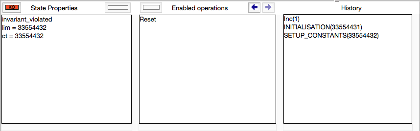
Symbolic Model Checking

Overview

The current nightly builds of ProB support different symbolic model checking algorithms:

• Bounded Model Checking (BMC),
• k-Induction, and
• different Variants of the IC3 algorithm.

As opposed to constraint-based checking, these algorithms find counterexamples which are reachable from the INITIALISATION. As opposed to ordinary model checking, they do not build up the state space explicitly, e.g., they do not compute all possible solutions for parameters and constants. This can be useful when the out-degree of the state-space is very high, i.e., when there are many possible solutions for the constants, the initialisation and/or the individual operations and their parameters.

In addition to the algorithms explained here, BMC*, a bounded model checking algorithm based on a different technique is available in Prob. See its wiki page for details.

Usage

Take the following example:

MACHINE VerySimpleCounterWrong
CONSTANTS lim
PROPERTIES lim = 2**25
VARIABLES ct
INVARIANT
 ct:INTEGER & ct < lim
INITIALISATION ct::0..(lim-1)
OPERATIONS
  Inc(i) = PRE i:1..1000 & ct + i <= lim THEN ct := ct+i END;
  Reset = PRE ct = lim THEN ct := 0 END
END

The ProB model checker will here run for a very long time before uncovering the error that occurs when ct is set to lim. If you run the TLC backend you will get the error message "Too many possible next states for the last state in the trace."

However, for the symbolic model checking techniques this is less of a problem. You can use them via command-line version of ProB as follows:

$ probcli VerySimpleCounterWrong.mch -symbolic_model_check bmc
K = 0
solve/2: result of prob: contradiction_found
K = 1
solve/2: result of prob: contradiction_found
K = 2
solve/2: result of prob: contradiction_found
K = 3
solve/2: result of prob: contradiction_found
K = 4
solve/2: result of prob: solution
successor_found(0)
 --> INITIALISATION(0)
successor_found(1)
 --> Inc
successor_found(2)
 --> Inc
successor_found(3)
 --> Inc
successor_found(4)
 --> Inc
! *** error occurred ***
! invariant_violation

Instead of "bmc" you can use "kinduction" and "ic3" as command line arguments in order to use the other algorithms.

The algorithms are also available from within ProB Tcl/Tk. They can be found inside the "Symbolic Model Checking" sub-menu of the "Analyse" menu.

More details

A paper describing the symbolic model checking algorithms and how they are applied to B and Event-B machines has been submitted to ABZ 2016.

Refinement Checking

Warning This page has not yet been reviewed. Parts of it may no longer be up to date

ProB can be used for refinement checking of B, Z and CSP specifications. Below we first discuss refinement checking for B machines. There is a tutorial on checking CSP assertions in ProB which can be viewed here.

What kind of refinement is checked?

ProB checks trace refinement. In other words, it checks whether every trace (consisting of executed operations with their parameter values and return values) of a refinement machine can also be performed by the abstract specification.

Hence, ProB does *not* check the gluing invariant. Also, PRE-conditions are treated as SELECT and PRE-conditions of the abstract machine are *not* always propagated down to the refinement machine. Hence, refinement checking has to be used with care for classical B machines, but it is well suited for EventB-style machines.

How does it work?

1. Open the abstract specification, explore its state space (e.g.,using an exhaustive temporal model check).
2. Use the command "Save state for later refinement check" in the "Verify" menu.
3. Open the refinement machine.
4. You can now use the "Refinement Check..." command in the "Verify" menu.

References

- ↑ M. Leuschel and E.Turner: Visualising larger state spaces in ProB. In H. Treharne, S. King, M. Henson, and S. Schneider, editors, ZB 2005: Formal Specification and Development in Z and B, LNCS 3455. Springer-Verlag, 2005 https://www3.hhu.de/stups/downloads/pdf/LeTu05_8.pdf
- ↑ O. Lichtenstein and A. Pnueli: Checking that Finite State Concurrent Programs Satisfy Their Linear Specification. POPL '85, Proceedings of the 12th ACM SIGACT-SIGPLAN Symposium on Principles of Programming Languages, ACM, 1985
- ↑ Michael Leuschel, Michael Butler, Corinna Spermann and Edd Turner: Symmetry Reduction for B by Permutation Flooding, Proceedings of the 7th International B Conference (B2007),2007,pp. 79-93,LNCS 4355,Springer, [1]
- ↑ Corinna Spermann and Michael Leuschel: ProB gets Nauty: Effective Symmetry Reduction for B and Z Models, Proceedings Symposium TASE 2008,June,2008,pp. 15-22,IEEE
- ↑ Michael Leuschel and Thierry Massart: ProB gets Nauty: Efficient Approximate Verification of B via Symmetry Markers, Proceedings International Symmetry Conference,Januar,2007,Verlag, [2]
- ↑ D. Jackson: Alloy: A lightweight object modeling notation. ACM Transactions Software Engineering and Methodology (TOSEM), 11(2):256–290, 2002.