Handbook/Visualisation
Graphical Viewer
Introduction
ProB can generate a wide range of visualizations for your models, e.g.:
- the statespace of a model
- the value of a particular formula
- various reduced representation of the statespace of a model
- one particular state of a model represented as a graph
Firstly, ProB generates a textual representation of a graph in the "dot" format. This information is typically saved to a file which has the same name and path as your main model but has a ".dot" extension. It then uses GraphViz to render this file. For this, it can either make use of the "dot" program to generate a Postscript file (generating a file with the ".ps" extension), or it uses a Dot-Viewer (such as "dotty") to view the file directly.
Setting up the Graphical Viewer
- GraphViz: in order to make use of the graphical visualization features, you need to install a version of GraphViz suitable for your architecture. More details can be found in Installation.
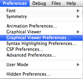
- Then use the command "Graphical Viewer Preferences..." in the "Preferences" Menu:

Then set or check the following preferences:
- Path/Command for dot program
- Path/Command for dot viewer (e.g., dotty)
Note: you can use the "Pick" button to locate the dot program and the dot viewer.
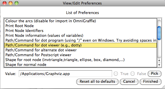

In case you want to use the Postscript option, also make sure that you have a viewer for Postscript files installed, and set the preference "Path/Command for Postscript viewer".
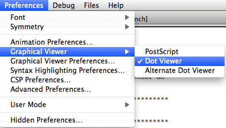
- You can select which viewer to use by going to the "Graphical Viewer" sub-menu of the "Preferences" Menu:
 .
.

State Space Visualization
ProB provides several user-friendly visualization features to help the user to analyze and understand the behavior of his B specification. This feedback is very beneficial to the understanding of the B specification since human perception is good at identifying structural similarities and symmetries. For more information on this particular topic, the reader can refer to [1] and [2].
In this page we discuss the visualization of the state space of a specification. Visualizing individual states can be visualized using animation functions, Custom_Graph definitions or using VisB.
The visualization features of the state space are in the "Visualize" menu, and comprise the command (visualize) "Statespace" and all the commands of the sub-menu "Statespace Projections". It is important to understand that those commands operate on the state space computed by ProB at the current point during the animation. Each time the user animates the B specification, the state space computed by ProB can be expanded if the selected operations lead to states not already computed by ProB. As shown in the following figure, the command (visualize) "Statespace" displays a diagram corresponding to the state space currently explored by the animation in a separate window.

Graph Nodes
ProB displays the state space as a graph whose nodes correspond to states that are differentiated by their shapes and colors and arcs correspond to operations. The operations are all those that are displayed in the Enabled Operations pane except backtrack, which is only useful for animation. Four types of nodes are visualized in ProB:
- root The point before the B machine is initialized when it has no state;
- current The current state during the animation;
- normal The states that have been already computed during the animation;
- open The states that are reachable from the normal states by an enabled operation.
In addition to its type, a node can indicate that it corresponds to an invariant violation, which is displayed by a color filling as shown in the following figure

Finally, if you have specified a goal predicate (either using a DEFINITION GOAL == P or by using a command such as "Find state satisfying predicate...") then those predicates are coloured in orange. Many of the colours and shapes can be changed by adapting the corresponding preferences. A list of preferences is now shown automatically in ProB Tcl/Tk.
Statespace Projections
The sub-menu "Statespace Projections" contains several other commands that provide useful views on the state space.
- Transition Diagram for Custom Expression ...
- Signature-Merge Reduced Statespace...
- DFA Reduced Statespace
- Subgraph leading to Invariant Violation
- Subgraph for GOAL
Transition Diagram
The first command allows you to enter an expression (in B syntax). The command will then merge all states with the same value for that expression into an equivalence class node. In other words, the state space is projected onto the values of the expression. The generated graph contains only transitions which change the value of that expression (unless the DOT_LOOPS preference is set to true). The command allows one to project the state space onto a single variable, a subset of variables (by using a tuple (v1,v2,...,vk) as expression). You can increase the projection by using B operators such as card, ran, dom or any other B operator. A more detailed explanation is given in [2]. The command can also be called from probcli using these commands (in conjunction with other commands like --model-check):
probcli -dotexpr transition_diagram EXPR DOTFILE
The generated dot file can be viewed with a viewer like dotty or can be converted, e.g., to PDF using:
dot -Tpdf <DOTFILE >PDFFILE
Here is an example where a faulty lift model has been projected onto the expression
curfloor / 3

Signature and DFA Merge
The two next commands in the menu "View Visited States|View" provide a means to display a simplified version of the state space. A more detailed explanation is given in [1].
The command "Signature-Merge Reduced Statespace" displays a state space where nodes sharing the same output arcs are collapsed into one node. The command "Reducted Deterministic Automaton of Visited States" removes the non-determinacy of the state space graph. The command "Select Operations & Arguments for Reduction" is used to specify which operations and arguments are affected by the previous transformations.
Sub Graphs
The two last commands of the "Statespace Projections" sub-menu display subgraphs of the state space. The command "Subgraph for Invariant Violation" displays the subgraph of nodes which violate the invariant, while the command "Subgraph of nodes satisfying GOAL" displays the subgraph where goals (discussed in Temporal Model Checking) are satisfied.
As of December 2015, there is also a sub-menu "Statespace Fast Rendering", which enables one to visualize larger state spaces more effectively. Some sample visualizations can be found here.
Other Visualization Commands
The "Visualize" menu contains several other sub-menus, to visualize traces and individual states. The command "Shortest Trace to Current State" displays the shortest sequence of nodes in the state space starting from the root node and leading to the current node. The command "Current State" displays the current node and its successor nodes.
Preferences of the Visualization
Many aspects of the visualization can be configured in the "Graphical Viewer Preferences"... preference window of the "Preferences" menu. This includes changing the shapes and colors of the various nodes (using the notation of the dot tool, see Dot-Shapes and Dot-Colors). For selecting the colors, a color picker is available via the button Pick. The user can also select which labels to display on the nodes (value of variables) and arcs (operation arguments and return value of functions), and their font size.
The default graph viewer in ProB is dotty, which is from the Graphviz package. ProB enables the user to display the graph using a PostScript viewer by setting the preference Use PostScript Viewer in the Graphical Viewer Preferences to true.... The PostScript file is generated by the dot tool. The path to the PostScript viewer can be set in the "Path/Command" for PostScript Viewer preference. The "Pick" button can be used to select the path. WARNING: All paths to files and folders should use the / character to separate the folders and should be absolute.
Using a postscript viewer rather than dotty has several advantages and several drawbacks. Firstly, the assignment of node shapes and colors is more accurately realized by dot (and therefore PostScript). Dotty on the other hand is much easier to use when state spaces are large thanks to the birds-eye view. A PostScript viewer also has the advantage that the PostScript file may be used to capture visualizations for publication purposes.
At present, the distinction between using a PostScript viewer as opposed to dotty comes down to the difference in functionality between the !GraphViz utilities dot and dotty. The main differences with respect to visualization in ProB are are:
- For Postscript: Support for more visualization shapes (for example, the shape double-octagon appears as a box on dotty);
- Against PostScript: dot does not support the addition of shapes to arcs. With moderately large graphs, Dot may put nodes outside of the printable or viewable area. Examining large graphs in a PostScript viewer may be slow (it may be awkward to use pan and zoom). There is less support for information on arcs (for example, dotted lines).
- For Dotty: Graphs can be modified. Dotty includes a birds-eye viewer which is useful for examining large graphs.
- Against Dotty: Dotty may crash if the graph is too big or complex (and on Solaris and Linux if non-standard mouse buttons are used).
References
- ↑ 1.0 1.1 M. Leuschel and E.Turner: Visualising larger state spaces in ProB. In H. Treharne, S. King, M. Henson, and S. Schneider, editors, ZB 2005: Formal Specification and Development in Z and B, LNCS 3455. Springer-Verlag, 2005 https://www3.hhu.de/stups/downloads/pdf/LeTu05_8.pdf
- ↑ 2.0 2.1 L. Ladenberger and M. Leuschel: Mastering the Visualization of Larger State Spaces with Projection Diagrams. ICFEM'2015, LNCS 9407. Springer-Verlag, 2015. https://www3.hhu.de/stups/downloads/pdf/LadenbergerLeuschel_ProjectDiagram.pdf
State space visualization examples
(This page is under construction)
Alternating Bit Protocol
This is a visualisation of 3643 states and 11115 transitions of a TLA+ model of the alternating bit protocol, as distributed with the TLA+ tools. This model (MCAlternatingBit.tla) was loaded with ProB for TLA+, the model checker run for a few seconds and then the command "State Space Fast Rendering" with options (scale,fast) was used.
The goal predicate rBit=1 was used; those states satisfying this predicate are shown in orange.

Below is a projection of this state space onto the expression (rBit,sBit), using the "Custom Transition Diagram" feature of ProB:

More details about this statespace projection feature can be found in our ICFEM'15 article.
The main file of the model is:
--------------------------- MODULE MCAlternatingBit -------------------------
EXTENDS AlternatingBit, TLC

INSTANCE ABCorrectness

CONSTANTS msgQLen, ackQLen

SeqConstraint == /\ Len(msgQ) \leq msgQLen
                 /\ Len(ackQ) \leq ackQLen

SentLeadsToRcvd == \A d \in Data : (sent = d) /\ (sBit # sAck) ~> (rcvd = d)
=============================================================================

ImpliedAction == [ABCNext]_cvars

TNext == WF_msgQ(~ABTypeInv')
TProp == \A d \in Data : (sent = d) => [](sent = d)

CSpec == ABSpec /\ TNext

DataPerm == Permutations(Data)
==============================================================
MCInnerFIFO
This is a visualisation of 3866 states and 9661 transitions of a TLA+ model of a FIFO, as distributed with the TLA+ tools. This model (MCInnerFIFO) was loaded with ProB for TLA+ and the model checker run so that all states with queue size greater than qLen (3) were ignored, i.e., no successor states were computed (this can be set by defining SCOPE==card(q)<=qLen). The colour indicates the length of the queue variable q of the model (gray=0,blue=1,red=2, green=3, lightgray=4) .

Below is a projection of this state space onto the expression card(q), using the "Custom Transition Diagram" feature of ProB:

RushHour
This is a visualisation of the Rush_Hour_Puzzle Rush Hour puzzle B model, at the moment that ProB has found a solution to the goal predicate (red car moved out of the grid). The solution node(s) are marked in orange and the prism option was used.

Here is a visualisation of the full state space of 4782 nodes and 29890 transitions, using the scale option this time:

CAN Bus
This is a visualisation of the statespace of an Event-B model of a CAN Bus. The colours indicate the size of the BUSwrite variable (gray=0,blue=1,red=2, green=3, lightgray=4).

Hanoi (6 Discs)
This is a visualisation of the statespace of a B model of the towers of Hanoi for 6 discs. The state space contains 731 nodes and 2186 nodes.

One can observe that this figure resembles a Sierpinski triangle. This is no coincidence, the state space of Hanoi is one.
Below is a projection of this state space onto the expression card(on(dest))), using the "Custom Transition Diagram" feature of ProB:

Threads - Partial Order Reduction
This is the visualisation of a simple threads model, of two threads with n=51 steps before a synchronisation occurs and threads start again. The state space contains 5410 nodes. One can clearly see two synchronisation points on the left-hand side and right-hand side, and that in between synchronisation the processes simply interleave.

With partial order reduction, the state space is reduced to 208 states:

Here is the B source code of the model:
MACHINE Threads51
/* Two simple threads communicating from time to time
This kind of situation should happen quite often in controller systems
A partial-order reduction can hopefully reduce the interleavings
*/
DEFINITIONS
 ASSERT_LTL1 == "F deadlock(Step1_p1,Step1_p2)";
 HEURISTIC_FUNCTION == pc1 // for sfdp colouring
CONSTANTS n
PROPERTIES n = 51 /* n=51: 208 states with POR (deadlock checking), 5410 without */
VARIABLES pc1,pc2, v1,v2
INVARIANT
pc1 : NATURAL & pc2:NATURAL &
v1 :  INTEGER & v2:INTEGER
INITIALISATION pc1,pc2,v1,v2 := 0,0,0,0
OPERATIONS
 Step1_p1 = PRE pc1<n THEN /* maybe the fact that we have a decreasing variant has an influence on POR ? In Event-B this event would be convergent */
     pc1 := pc1+1|| v1 := v1+1
 END;
 Step1_p2 = PRE pc2<n /* & pc1=n manual POR */
             THEN /* also a convergent event (variant n-pc2) */
     pc2 := pc2+1 || v2 := v2+1
 END;
 Sync = PRE pc1=n & pc2=n THEN
    pc1, pc2 := 0,0 ||
    v1,v2 := v1 mod 2, v2 mod 2
 END
END
Below are projections of the above state spaces onto the expression (bool(pc1=n),bool(pc2=n)), using the "Custom Transition Diagram" feature of ProB.
The first shows the projection without partial order reduction:

With partial order reduction, one can see that the Step1_p1 events now all occur before the Step1_p2 events:

Eval Console
For this tutorial, load for example the file StackConstructive.mch included in the examples/Tutorial directory of the ProB distribution (this example is also discussed in the Tutorial Modeling Infinite Datatypes).
After loading the file, double click on the green line "SETUP_CONSTANTS" in the "Enabled Operations" pane. Now double click on the green "INITIALISATION" line in the same pane. To start the "Eval..." interactive console you can either
- use the "Eval..." command in the Analyse menu,
- double-click any line in the "State Properties" pane or
- right-click (Control-Click on a Mac) on the "State Properties" pane and select the "Eval..." entry as shown below:

This will bring up a new window, the "Eval Console":

You can now enter predicates or expressions and hit return or enter to evaluate them in the current state of the machine. Below is a small transcript:

You can use the up and down arrow keys to navigate to earlier predicates or expressions you have entered.
If you change the state, then the expressions and predicates are evaluated in that state. For example, if you execute the operations Push(RANGE3), Push(RANGE1), Push(RANGE2) by double-clicking on the respective lines in the "Enabled Operations" pane, then a transcript of using the console is as follows:

The console works the same way for Event-B models, Z and TLA specifications. However, in all those cases the Eval console uses the classical B parser and you have to use classical B syntax for entering predicates or expressions. The console also works in CSP mode and uses a CSP parser there.
As of version 1.4 the console allows defining new local variables (local to the console) using Haskell's let syntax: let id = Expr. You can use the :b command to browse your let definitions. Here is an example session:
>>> let x = 2**10
 1024
>>> let y = x+x
 2048
>>> :b
  x = 1024
  y = 2048
>>> {v| v>x & v<y & v mod x = 1}
 {1025}
>>>
A similar console is also available for the command-line version of ProB (probcli) using the -repl command. More details are available on the separate wiki page for probcli.
We now also have made two versions of a ProB Logic Calculator available online. The second one works similarly to the Eval console above, but is not linked to any B machine. You can try it out directly on this page below:
Evaluation View
This tutorial describes the use of ProB's evaluation view to explore single states of a model. The view shows the details of a particular state during the animation. It can be used to
- learn about the values of a some variables. This feature is overlapping with the State Properties View in the bottom left section of ProB's main window, but the evaluation view allows to inspect a value in greater detail.
- understand the truth value of the invariant and its sub-formulas and the values of the sub-expressions.
- export the content of variables in a state to use them outside of ProB.
Inspecting the State Variables and Constants
As an example specification we use the Sieve.mch delivered with the ProB Distribution in the "Less Simple" folder. After opening the model do a couple of animation steps and then open the Evaluation view in the Analyse menu. You should get window that looks similar to the following screenshot:

You can now expand each of the three sections to investigate the current state of the machine. For instance if we expand the Variables section we will get the following:

The tree shows values for each variable in the same way as the State Properties view. The value of the variable numbers in our example tell us that card(numbers) = 2288 and it shows the first and last entries. In contrast to the State Properties View you can see all values by doubleclicking an entry as shown in the next screenshot.

The save button can be used to save the value of the variable (as a B-Expression) to a file. You can also save the values of multiple variables (we will cover this later).
Understanding the Invariant and Properties
The second objective of the evaluation view is to help understanding why the invariant or the properties are true or false. Therefore the view allows us to expand a predicate into its sub-predicates and sub-expressions. This can be demonstrated using Priorityqueue.mch from the folder SchneiderBook. After initializing the machine and a few animation-steps opening the evaluation view yields

The invariant consists of two predicates
- queue : seq(NAT)
- !xx . (xx : 1..size(queue)-1 => (queue(xx) <= queue(xx+1)))
The first invariant is very simple. It is a predicate that has two sub-expressions queue and seq(NAT). The view shows the values for both subexpressions. Note that seq(NAT) is kept symbolic. The second invariant is more complex. It consistis of a sub-expression xx and and implication which has two sub-predicates xx : 1..size(queue)-1 and queue(xx) <= queue(xx+1)). As we see, the sub-predicates can also be expanded until we reach the level of simple values. The value of xx is chosen arbitrarily because the universal quantification is true. So let us modify the machine and introduce a bug e.g.
 insert(nn) =
 PRE nn : NAT
 THEN
   SELECT queue = <> THEN queue := [nn]
   WHEN queue /= <> & nn <= min(ran(queue)) THEN queue := queue <- nn /*<-- the bug */
   WHEN queue /= <> & nn >= max(ran(queue)) THEN queue := queue <- nn
   ELSE ANY xx
        WHERE xx : 1..size(queue)-1 & queue(xx) <= nn & nn <= queue(xx+1)
        THEN queue := (queue /|\ xx) ^ [nn] ^ (queue \|/ xx)
        END
   END
 END;
Now we can model check the machine and ProB will find a state that violates the invariant. Opening the evaluation view gives us something like

In the case that a universal quantification predicate yields false, ProB gives us a counterexample. For existential quantification the result is dual. If the predicate is true, we will get a witness, if it is false, we will get an arbitrarily chosen example.
In addition ProB has some built-in rules that allows us to better see, why a predicate has failed. For instance the predicate A <: B will contain a constructed sub-predicate B-A={}. If the original predicate is violated, then B - A it will contain precisely those elements that contradict the predicate. This makes it easy to spot the problem in particular if A and B are large sets. The behavior can be observed, for example, in the Paperround.mch model from the SchneiderBook folder. After a couple of operations the evaluation view looks like
If we introduce an error, such as
remove(hh) =
  PRE hh : 1..163
  THEN  papers := papers - {hh}
  END
we can now model check the machine and find a counter example that can be inspected using the evaluation view and because of the automatically introduced predicate it is very easy to see the reason why magazines <: papers is false.

Filtering relevant information and Data Extraction
There are two different ways to filter out important information from a state. To demonstrate this feature we can use the model SATLIB_blocksworld_medium.mch from the LessSimple folder of the ProB distribution. After executing SETUP_CONSTANTS and INITIALISATION we open the evaluation view. It contains a large number of constants and properties that might not be equally interesting.
The first way to filter out information is using the Search Box in the upper right part of the view. As we type, ProB will filter out all items that do not contain our search phrase. If we, for instance, type x19. We will get only those constants and properties that contain x19.

The second way to filter out unnecessary information is to mark some items and restrict the view. Suppose we are only interested in the constants x1, x4, x17 and the property (x4 = FALSE or X2=FALSE) or X6=TRUE (the first property in the list). Using the right mouse button, we can mark all the rows in the view that we want to see by selecting "Mark all selected items" from the context menu. In the same popup menu, we can select "Show only marked items" which will remove all other information.

Finally the popup menu allows us to save the content of a particular state into a file (either the full state, or the marked items only). In either case, ProB will generate a text file containing the state as a predicate. In our example the file will contain the following predicate
x1 = FALSE
 &
x4 = TRUE
 &
x17 = TRUE
 &
(x4 = FALSE or x2 = FALSE) or x6 = TRUE
Graphical Visualization
The graphical visualization of ProB [1] enables the user to easily write custom graphical state representations in order to provide a better understanding of a model. With this method, one assembles a series of pictures and writes an animation function in B. Each picture can be associated to a specific state of a B variable or expression. Then, depending on the current state of the model, the animation function in B stipulates which pictures should be displayed where. We now show how this animation can be done with very little effort.
As an alternative you can also specify CUSTOM_GRAPH definitions to render the current state as graph laid out by GraphViz. In addition, ProB also supports more powerful visualizations based on SVG and HTML in the form of VisB.
The Graphical Animation Model
The animation model is very simple. It is based on individual images and a user-defined animation function, which are both defined in the DEFINITIONS section of the animated machine as follows:
1. Each image is given a number and its source file location by using the following definition:
ANIMATION_IMGx == "filename", where x is the number of the image and "filename" is its path to a gif image file.
2. A user-defined animation function fa is evaluated to recompute the graphical output for every state. The graphical output of fa is known as the graphical visualization, which consists of a two-dimensional grid. Each cell in the grid can contain an image. The function uses the variables r (for row) and c (for column) to determine in which cell the image will be displayed. An image can appear multiple times in the grid.
The function fa is declared by defining ANIMATION_FUNCTION and ideally should be of type INTEGER * INTEGER +-> INTEGER. If the function fa is defined for r and c, then the animator should display the image with number fa(r,c) at row r and column c. If the function is undefined at this position, no image is displayed in the corresponding cell.
Notes: ProB will try and convert your expression to INTEGER * INTEGER +-> INTEGER (see below). Instead of an ANIMATION_IMGx one can also declare ANIMATION_STRx definitions for textual representations. If there is no image or string definition for the number fa(r,c) or if fa(r,c) is no number then ProB will try and display the result in pretty-printed textual format.
The dimension of the grid is computed by examining the minimum and maximum coordinates that occur in the animation function. More precisely,
the rows are in the range min(dom(dom(fa)))..max(dom(dom(fa))) and
the columns are in the range min(ran(dom(fa)))..max(ran(dom(fa))).
We take the B machine of the sliding 8-puzzle as an example. In the 8-puzzle, the tiles are numbered. Every tile can be moved horizontally and vertically into an empty square. The final configuration is reached whenever all the tiles are in order.
The B machine of the 8-puzzle is as follows:
MACHINE Puzzle8
DEFINITIONS INV == (board: ((1..dim)*(1..dim)) -->> 0..nmax);
GOAL == !(i,j).(i:1..dim & j:1..dim => board(i|->j) = j-1+(i-1)*dim);
CONSTANTS dim, nmax
PROPERTIES dim:NATURAL1 & dim=3 & nmax:NATURAL1 & nmax = dim*dim-1
VARIABLES board
INVARIANT INV
INITIALISATION board : (INV & GOAL)
OPERATIONS
 MoveDown(i,j,x) = PRE i:2..dim & j:1..dim &
                       board(i|->j) = 0 & x:1..nmax & board(i-1|->j) = x
                   THEN board := board <+ {(i|->j)|->x, (i-1|->j)|->0}
                   END;
 MoveUp(i,j,x) = PRE i:1..dim-1 & j:1..dim &
                          board(i|->j) = 0 & x:1..nmax & board(i+1|->j) = x
                 THEN board := board <+ {(i|->j)|->x, (i+1|->j)|->0}
                 END;
 MoveRight(i,j,x) = PRE i:1..dim & j:2..dim &
                        board(i|->j) = 0 & x:1..nmax & board(i|->j-1) = x
                    THEN board := board <+ {(i|->j)|->x, (i|->j-1)|->0}
                    END;
 MoveLeft(i,j,x) = PRE i:1..dim & j:1..dim-1 &
                       board(i|->j) = 0 & x:1..nmax & board(i|->j+1) = x
                   THEN board := board <+ {(i|->j)|->x, (i|->j+1)|->0}
                   END
END
On the left side of the following Figure, the non-graphical visualization is generated by ProB. It is readable, but the graphical visualization at the right side is much easier to understand.

The graphical visualisation is achieved with very little effort by writing in the DEFINITIONS section, the following animation function, as well as the image declaration list:
ANIMATION_FUNCTION == ( {r,c,i|r:1..dim & c:1..dim & i=0} <+ board);
ANIMATION_IMG0 == "images/sm_empty_box.gif"; /* empty square */
ANIMATION_IMG1 == "images/sm_1.gif"; /* square with 1 inside */
ANIMATION_IMG2 == "images/sm_2.gif";
ANIMATION_IMG3 == "images/sm_3.gif";
ANIMATION_IMG4 == "images/sm_4.gif";
ANIMATION_IMG5 == "images/sm_5.gif";
ANIMATION_IMG6 == "images/sm_6.gif";
ANIMATION_IMG7 == "images/sm_7.gif";
ANIMATION_IMG8 == "images/sm_8.gif"; /* square with lightblue 8 inside */
Each of the three integer types in the signature can be replaced by a deferred or enumerated set, in which case our tool translates elements of this set into numbers. In the case of enumerated sets, the number is the position of the element in the definition of the set in the SETS clause. Deferred set elements are numbered internally by ProB, and this number is used. (Note however, that the whole animation function has to be of the same type; otherwise the animator will complain about a type error.) To avoid having to produce images for simple strings, one can use a declaration ANIMATION_STRx == "my string" to define image with number x to be automatically generated from the given string.
Typical patterns for the animation function are as follows:
- A useful way to obtain a function of the required signature is to write a set comprehension of the following form:
{row,col,img | row:1..NrRow & col:1..NrCols & P},
 where P is a predicate which gives img a value depending on row and col.
- Another useful pattern is to write one function for default images and then use the override operator to replace the default images only when needed:
DefaultImages <+ CurrentImages
This was used in the 8-Puzzle by setting as default the empty square (image 0), which is then overriden by the partially defined board function.
- or to write multiple definitions of the animation function. More clearly, we define one animation function for default images and another one for current images as follows:
ANIMATION_FUNCTION_DEFAULT == DefaultImages;
ANIMATION_FUNCTION == CurrentImages;
Note: as of version 1.4 of ProB you can define multiple animation functions (e.g., ANIMATION_FUNCTION1, ANIMATION_FUNCTION2, ...) each overriding its predecessor.
This was used next in the Sudoku example.
- Translation Predicates between user sets and numbers (extension above can directly handle user sets but does not work well if we need a special image for undefined,...)
Further Examples
Below we illustrate how the graphical animation model easily provides interesting animations for different models.
Scheduler
The scheduler specification taken from [2] is as follows:
MACHINE scheduler
SETS PID = {process1,process2,process3}
VARIABLES active, ready, waiting
INVARIANT active <: PID & ready <: PID & waiting <: PID &
          (ready /\ waiting) = {} & active /\ (ready \/ waiting) = {} &
          card(active) <= 1 & ((active = {}) => (ready = {}))
INITIALISATION active := {} || ready := {} || waiting := {}
OPERATIONS
 new(pp) =
  SELECT pp : PID & pp /: active & pp /: (ready \/ waiting)
  THEN waiting := (waiting \/ { pp })
  END;
 del(pp) =
  SELECT pp : waiting
  THEN waiting := waiting - { pp }
  END;
 ready(rr) =
  SELECT rr : waiting
  THEN waiting := (waiting - {rr}) ||
       IF (active = {})
       THEN active := {rr}
       ELSE ready := ready \/ {rr}
       END
  END;
 swap =
  SELECT active /= {}
  THEN waiting := (waiting \/ active) ||
       IF (ready = {}) THEN active := {}
       ELSE
        ANY pp WHERE pp : ready
        THEN active := {pp} || ready := ready - {pp}
        END
       END
  END
END
The left side of the following Figure shows the non-graphical animation of the machine scheduler, and the right side shows its graphical animation obtained using ProB.

The graphical visualization is done by writing in the DEFINTIONS section the following animation function. Here, we need to map PID elements to image numbers.
IsPidNrci == p=process1 & i=1) or (p=process2 & i=2) or (p=process3 & i=3));
ANIMATION_FUNCTION ==
 ({1|->0|->5, 2|->0|->6, 3|->0|->7} \/ {r,c,img|r:1..3 & img=4 & c:1..3} <+
 ({r,c,i| r=1 & i:INTEGER & c=i & #p.(p:waiting & IsPidNrci)} \/
 {r,c,i| r=2 & i:INTEGER & c=i & #p.(p:ready & IsPidNrci)} \/
 {r,c,i| r=3 & i:INTEGER & c=i & #p.(p:active & IsPidNrci)} ));
ANIMATION_IMG1 == "images/1.gif";
ANIMATION_IMG2 == "images/2.gif";
ANIMATION_IMG3 == "images/3.gif";
ANIMATION_IMG4 == "images/empty_box.gif";
ANIMATION_IMG5 == "images/Waiting.gif";
ANIMATION_IMG6 == "images/Ready.gif";
ANIMATION_IMG7 == "images/Active.gif"
The previous animation function of scheduler can also be rewritten as follows:
ANIMATION_FUNCTION_DEFAULT ==
 ( {1|->0|->5, 2|->0|->6, 3|->0|->7} \/ {r,c,img|r:1..3 & img=4 & c:1..3} );
ANIMATION_FUNCTION == ({r,c,i| r=1 & i:PID & c=i & i:waiting} \/
                       {r,c,i| r=2 & i:PID & c=i & i:ready} \/
                       {r,c,i| r=3 & i:PID & c=i & i:active}
                      );
Sudoku
Using ProB we can also solve Sudoku puzzles. The machine has the variable Sudoku9 of type 1..fullsize-->(1..fullsize+->NRS), where NRS is an enumerate set {n1, n2, ...} of cardinality fullsize.
The animation function is as follows:
Nri == ((Sudoku9(r)(c)=n1 => i=1) & (Sudoku9(r)(c)=n2 => i=2) &
        (Sudoku9(r)(c)=n3 => i=3) & (Sudoku9(r)(c)=n4 => i=4) &
        (Sudoku9(r)(c)=n5 => i=5) & (Sudoku9(r)(c)=n6 => i=6) &
        (Sudoku9(r)(c)=n7 => i=7) & (Sudoku9(r)(c)=n8 => i=8) &
        (Sudoku9(r)(c)=n9 => i=9)
       );
ANIMATION_FUNCTION == ({r,c,i|r:1..fullsize & c:1..fullsize & i=0} <+
                       {r,c,i|r:1..fullsize & c:1..fullsize &
                       c:dom(Sudoku9(r)) & i:1.. fullsize & Nri}
                      );
The following Figure shows the non-graphical visualization of a particular puzzle (left), the graphical visualization of the puzzle (middle), as well as the visualization of the solution found by ProB after a couple of seconds (right).

Note that it would have been nice to be able to replace Nri inside the animation function simply by i = Sudoku9(r)(c). While our visualization algorithm can automatically convert set elements to numbers, the problem is that there is a type error in the override: the left-hand side is a function of type INTEGER*INTEGER+->INTEGER, while the right-hand side now becomes a function of type INTEGER*INTEGER+->NRS. One solution is to write multiple definitions of the animation function. In addition to the standard animation function, we can define a default background animation function. The standard animation function will override the default animation function, but the overriding is done within the graphical animator and not within a B formula. In this way, one can now rewrite the above animation as follows:
ANIMATION_FUNCTION_DEFAULT == ( {r,c,i|r:1..fullsize & c:1..fullsize & i=0} );
ANIMATION_FUNCTION == ({r,c,i|r:1..fullsize & c:1..fullsize &
                       c:dom(Sudoku9(r)) & i:1.. fullsize & i = Sudoku9(r)(c)}
                      )
Other Features
One can define actions for right clicks and mouse clicks and drags:
ANIMATION_RIGHT_CLICK(col,row) == SUBSTITUTION

ANIMATION_CLICK(fromcol,fromrow,tocol,torow) == SUBST
The allowed substitutions are currently limited:
- ANY, LET: to introduce wild cards; predicates will not (yet) be evaluated !!
- IF-ELSIF-ELSE: conditions have to be evaluable using the parameters only
- CHOICE: to provide multiple right click actions
One can set the font being used using ProB preferences. The following leads to a Monospaced font being used, making lining up of columns easier:
  SET_PREF_TK_CUSTOM_STATE_VIEW_FONT_NAME == "Monaco";
  SET_PREF_TK_CUSTOM_STATE_VIEW_FONT_SIZE == 9;
The following preferences can be used to control padding around cells:
  SET_PREF_TK_CUSTOM_STATE_VIEW_STRING_PADDING == Nr
  SET_PREF_TK_CUSTOM_STATE_VIEW_PADDING == Nr
The following preference can be used to disable the custom graphical visualization view:
SET_PREF_TK_CUSTOM_STATE_VIEW_VISIBLE == FALSE
One can control justification of animation strings using either of the two following DEFINITIONS:
ANIMATION_STR_JUSTIFY_LEFT == TRUE
ANIMATION_STR_JUSTIFY_RIGHT == TRUE
References
- ↑ M. Leuschel, M. Samia, J. Bendisposto and L. Luo: Easy Graphical Animation and Formula Viewing for Teaching B. In C. Attiogbé and H. Habrias, editors, Proceedings: The B Method: from Research to Teaching, pages 17-32, Nantes, France. APCB, 2008.
- ↑ B. Legeard, F. Peureux, and M. Utting. Automated boundary testing from Z and B. Proceedings of FME’02, LNCS 2391, pages 21–40. Springer-Verlag, 2002.