Tutorial LTL Counter-example View
In this tutorial a quick overview will be given describing the LTL counter-example visualization plug-in in Rodin. The functionality of the plug-in will be presented by means of an Event-B model on which different properties will be checked that are not satisfied by the model.
LTL Model Checking and the Meaning of Counter-examples
Model checking is a technique for checking in an automatic way whether a model satisfies a property expressed in formal logic. LTL (standing for linear temporal logic) is a version of the temporal logic used mainly for encoding time-dependent properties of systems.
Verifying whether a system fulfills an LTL property by means of model checking is realized by searching a path in the state space of the system that violates the property being checked. That is, if the system behaves in a way violating the LTL property being checked, then the erroneous behavior will be reported by returning a path (mostly infinite) representing the false behavior. Otherwise, if no counter-example was found, it will be considered that the system satisfies the LTL property.
The LTL model checker of ProB provides three types of counter-examples:
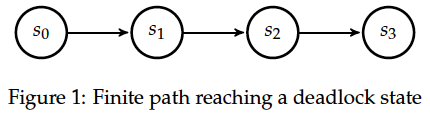
- Finite path leading to a deadlock state (see Figure 1):
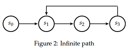
- Infinite path (see Figure 2), the infinite path in this case is represented by means of a loop:
- Finite path (see Figure 3). (In this case an infinite path representing the respective counter-example has been shortened in order to attract the attention to the relevant part of the counter-example).
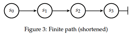


The first two types of counter-examples (Figure 1 and Figure 2) constitute a violation of a liveness[1] property, whereas the path in Figure 3 represents usually a counter-example for a safety property.
Visualization of Counter-examples in Rodin
Each state of a path in the LTL counter-example view is marked by a respective color that denotes the evaluation of an LTL formula at that state. There are three possible statuses (colors) that a state s may have in respect to an LTL formula f:
- Green: the value of f is true at s
- Red: the value of f is false at s
- Grey: the value of f cannot be determined at s (unknown value)
A state will be colored in grey if the value of the respective LTL formula cannot be determined. This may happen in case the counter-example is represented by finite path. For example, evaluating the LTL formula ‘X {p2=crit2}’ on a path of length two where the value of p2 is not equal to crit2 in both states (see Figure 4) yields the following coloring of the states in Rodin: [2]

Since the value of the atom ‘{p2=crit2}’ in is equal to false the value of the LTL formula ‘X {p2=crit2}’ in is also equal to false. Therefore the first state is colored in red. On the other hand, the value of the formula ‘X {p2=crit2}’ in is unknown as there is no successor state of in the path showed in Figure 4. Accordingly, the second state in the LTL counter-example viewer will be colored in grey.

States in the path considered to be significant for the evaluation of the respective LTL formula are highlighted by bright colors. Accordingly, the other states will be grayed out.
Consider the path in Figure 5 that can be reported as a counter-example for the LTL formula ‘{p1=noncrit1} U {p1=crit1}’. [3] As a result the LTL counter-example view will display the following visualization of the counter-example:

The path in Figure 5 violates ‘{p1=noncrit1} U {p1=crit1}’ since the goal (‘{p1=crit1}’) of the until-formula does not hold in all states of the path. This is illustrated by means of the bottom colored path in the picture above. Both states have been colored with bright red as both are significant for the violation of the until-formula in regard to ‘{p1=crit1}’.
The upper path in the picture above has been evaluated and colored in regard to the condition (‘{p1=noncrit1}’) of the until-formula. The critical state here is the second one as ‘{p1=noncrit1}’ does not hold in that state and therefore is it highlighted by a brighter color. On the other hand, the atom ‘{p1=noncrit1}’ holds in and thus the state is colored in green. has been grayed out since the evaluation of ‘{p1=noncrit1}’ in that state has no significant meaning for the violation of ‘{p1=noncrit1} U {p1=crit1}’.

Notice, for a given LTL formula f the values (or the colors) of the states are set in regard to the evaluation of the sub-formula/-s of f and highlighted with respect to the semantics of f. In case of the formula ‘{p1=noncrit1} U {p1=crit1}’ the states are colored in regard to the atoms ‘{p1=noncrit1}’ and ‘{p1=crit1}’ and highlighted in regard to the semantics of the until-operator.
A path reported as a counter-example of an LTL formula represents a possible trace of the model being analyzed. In some cases it may be helpful to know which transitions are executed along the path in order to reproduce the erroneous behavior of the model (e.g. by animating the trace). To see which transitions are being executed in the counter-example hold the mouse cursor on the respective edge. A label will come up with the transition name:

Another way to find out the transitions of the path is to inspect the current trace loaded in the history view.
To view a state of a counter-example showed in the LTL counter-example view perform a double-click action on the respective state. After double-clicking a state the relevant information (variables’ evaluation, invariant evaluation, etc.) of the state is displayed in the state view and the trace leading to the double-clicked state is loaded in the history view.
The counter-example reported by the LTL model checker will be visualized in regard to all operators used in the LTL formula. For example, three different visualizations will be illustrated for ‘G ({p1=wait1} => F {p1=crit1})’ as shown in the picture below. [4]:

In order to view the visualizations of the sub-formulas, one should click on one of the states of the source-formula.
References and Notes
- ↑ The first type of a counter-example (Figure 1) can in some cases be a valid counter-example for safety properties. For example, if the model cannot perform any actions, then a path possessing only single state is a counter-example for each LTL formula , with .
- ↑ The visualization refers to the LTL formula ‘XX {p2=crit2}’. However, in this example we are interested in the coloring of the states in regard to the LTL formula ‘X {p2=crit2}’.
- ↑ An LTL formula is satisfied by a path if there exists a state in fulfilling and holds at all states of until is reached.
- ↑ There are five sub-formulas for ‘G ({p1=wait1} => F {p1=crit1})’: ‘G ({p1=wait1} => F {p1=crit1})’, ‘{p1=wait1} => F {p1=crit1}’, ‘{p1=wait1}’, ‘F {p1=crit1}’, and ‘{p1=crit1}’. However, the number of visualizations corresponds not to the number of sub-formulas, but to the number of the operators used in the LTL formula.