Evaluation View: Difference between revisions

This tutorial describes the use of ProB's evaluation view to explore single states of a model. The view shows the details of a particular state during the animation. It can be used to

1. learn about the values of a some variables. This feature is overlapping with the State Properties View in the bottom left section of ProB's main window, but the evaluation view allows to inspect a value in greater detail.
2. understand the truth value of the invariant and its sub-formulas and the values of the sub-expressions.
3. export the content of variables in a state to use them outside of ProB.

Inspecting the State Variables and Constants

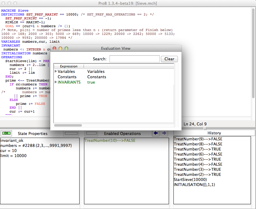
As an example specification we use the Sieve.mch delivered with the ProB Distribution in the "Less Simple" folder. After opening the model do a couple of animation steps and then open the Evaluation view in the Analyse menu. You should get window that looks similar to the following screenshot:

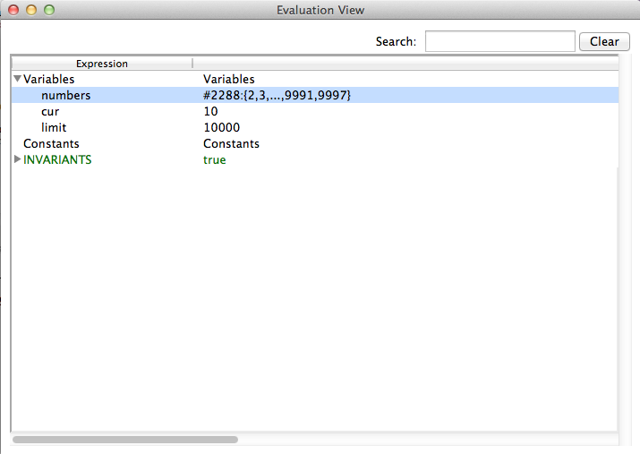
You can now expand each of the three sections to investigate the current state of the machine. For instance if we expand the Variables section we will get the following:

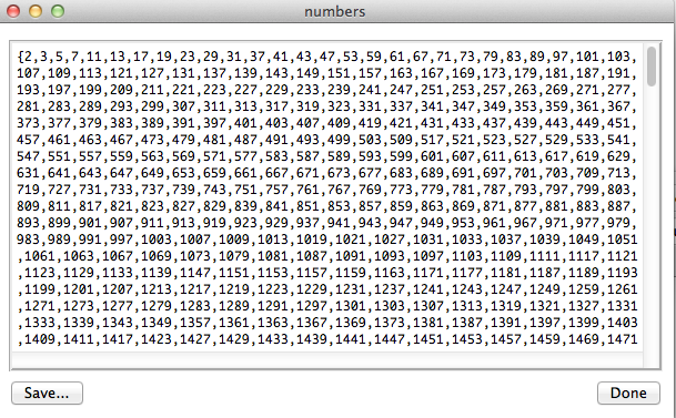
The tree shows values for each variable in the same way as the State Properties view. The value of the variable numbers in our example tell us that card(numbers) = 2288 and it shows the first and last entries. In contrast to the State Properties View you can see all values by doubleclicking an entry as shown in the next screenshot.

The save button can be used to save the value of the variable (as a B-Expression) to a file. You can also save the values of multiple variables (we will cover this later).

Understanding the Invariant and Properties

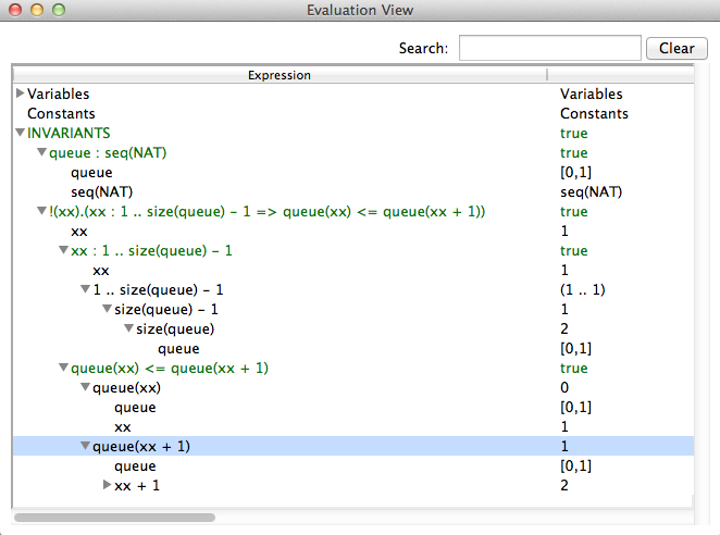
The second objective of the evaluation view is to help understanding why the invariant or the properties are true or false. Therefore the view allows us to expand a predicate into its sub-predicates and sub-expressions. This can be demonstrated using Priorityqueue.mch from the Folder SchneiderBook. After initializing the machine and a few animation-steps opening the evaluation view yields

The invariant consists of two predicates

1. queue : seq(NAT)
2. !xx . (xx : 1..size(queue)-1 => (queue(xx) <= queue(xx+1)))

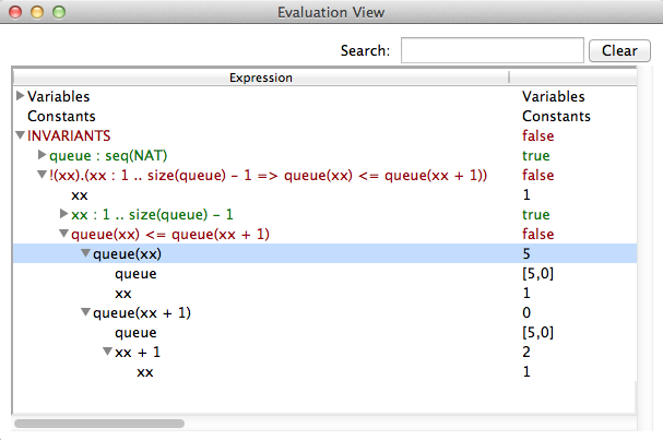
The first invariant is very simple. It is a predicate that has two sub-expressions queue and seq(NAT). The view shows the values for both subexpressions. Note that seq(NAT) is kept symbolic. The second invariant is more complex. It consistis of a sub-expression xx and and implication which has two sub-predicates xx : 1..size(queue)-1 and queue(xx) <= queue(xx+1)). As we see, the sub-predicates can also be expanded until we reach the level of simple values. The value of xx is chosen arbitrarily because the universal quantification is true. So let us modify the machine and introduce a bug e.g.

 insert(nn) =
 PRE nn : NAT
 THEN 
   SELECT queue = <> THEN queue := [nn]
   WHEN queue /= <> & nn <= min(ran(queue)) THEN queue := queue <- nn /*<-- the bug */
   WHEN queue /= <> & nn >= max(ran(queue)) THEN queue := queue <- nn
   ELSE ANY xx
        WHERE xx : 1..size(queue)-1 & queue(xx) <= nn & nn <= queue(xx+1)
        THEN queue := (queue /|\ xx) ^ [nn] ^ (queue \|/ xx)
        END
   END
 END;

Now we can model check the machine and ProB will find a state that violates the invariant. Opening the evaluation view gives us something like

In the case that a universal quantification predicate yields false, ProB gives us a counterexample. For existential quantification the result is dual. If the predicate is true, we will get a witness, if it is false, we will get an arbitrarily chosen example.

In addition ProB has some built-in rules that allows us to better see, why a predicate has failed. For instance the predicate A <: B will contain a constructed sub-predicate B-A={}. If the original predicate is violated, then the result of B-A will clearly show why A is not a subset of B, it will contain precisely those elements that contradict the predicate.

Filtering relevant information

Data Extraction