B2SAT: Difference between revisions
No edit summary |
|||
| Line 121: | Line 121: | ||
=== B2SAT in Jupyter Notebooks === | === B2SAT in Jupyter Notebooks === | ||
The solve command in the ProB Jupyter kernel now supports <tt>sat</tt> and <tt>satz3</tt> as solvers. | The solve command in the https://gitlab.cs.uni-duesseldorf.de/general/stups/prob2-jupyter-kernel ProB Jupyter kernel now supports <tt>sat</tt> and <tt>satz3</tt> as solvers. | ||
They use B2SAT with Glucose and Z3 as SAT solvers respectively. | They use B2SAT with Glucose and Z3 as SAT solvers respectively. | ||
Revision as of 07:40, 24 April 2024
The current versions of ProB can make use of the new B2SAT backend as an alternate way of solving constraints. It translates a subset of B formulas to SAT and for solving by an external SAT solver. The new backend interleaves low-level SAT solving with high-level constraint solving performed by the default solver of ProB.
B2SAT solving consists of the following phases:
- the deterministic propagation phase(s) of ProB's solver: it performs deterministic propagations and can expand quantifiers and total functions.
- a compilation phase, whereby static values are inlined.
- the B to CNF conversion proper, which can translate a subset of B to propositional logic in conjunctive normal form. This phase currently supports:
- equalities and inequalities between boolean variables and constants,
- all logical connectives and
- some cardinality constraints.
- Subformulas that cannot be solved are sent to ProB's default solver and linked to the CNF via an auxiliary propositional variable.
- solving phase, where the generated CNF is sent to an external SAT solver.
- propagation of the SAT solution to B, by progressively grounding the B values and predicates linked to the propositional variables.
- complete constraint solving, solving the pending constraints in B by now performing the regular non-deterministic propagations and enumerations of ProB.
Using B2SAT
B2SAT in the REPL
The following four commands are now available in REPL of probcli (start with probcli --repl):
- :sat PRED
- :sat-z3 PRED
- :sat-double-check PRED
- :sat-z3-double-check PRED
Here is a simple example:
 >>> :sat f:1..n --> BOOL & n=3 & f(1)=TRUE & !i.(i:2..n => f(i) /= f(i-1))
 PREDICATE is TRUE
 Solution:
        f = {(1|->TRUE),(2|->FALSE),(3|->TRUE)} &
        n = 3
B2SAT for PROPERTIES
The new preference SOLVER_FOR_PROPERTIES can be used to specify solver for PROPERTIES (axioms) when setting up constants. The valid settings are: prob (the default), kodkod, z3, z3cns, z3axm, cdclt, sat, sat-z3.
The last two will use B2SAT, sat with Glucose as SAT solver and sat-z3 with Z3 as SAT solver.
Here is an example using this preference to compute a dominating set of a graph:
MACHINE IceCream_Generic
// Dominating set example:
// place ice cream vans so that every house (node) is at most one block away from a van
DEFINITIONS
  N == 24;
  CUSTOM_GRAPH == rec(layout:"dot", rankdir:"TB",
                     nodes: {j•j:NODES |
                               rec(value:j, style:"filled",
                                fillcolor:IF ice(j)=TRUE THEN "mistyrose" ELSE "white" END
                                  )},
                    edges:rec(color:"gray", arrowhead:"odot",
                              arrowtail:"odot", dir:"both",
                              label:"edge",   edges: edge)
                    );
      bi_edge == (edge \/ edge~);
  SET_PREF_SOLVER_FOR_PROPERTIES == "sat";
SETS
  NODES = {n1,n2,n3,n4,n5,n6,n7,n8,n9,n10,
           n11,n12,n13,n14,n15,n16,n17,n18,n19,n20,n21,n22,n23,n24}
CONSTANTS edge, ice, vans, neighbours
PROPERTIES
 edge: NODES <-> NODES &
 edge = { n1|->n2, n1|->n4,
          n2|->n3,
          n3|->n4, n3|->n5, n3|->n7,
          n4|->n7,
          n5|->n6, n5|->n9,
          n6|->n7, n6|->n8,
          n7|->n8,
          n8|->n10, n8|->n13,
          n9|->n10, n9|->n11, n9|->n12,
          n11|->n12, n11|->n14,
          n12|->n13,
          n13|->n16,
          n14|->n15, n14|->n17,
          n15|->n16, n15|->n17, n15|->n18, n15|->n21,
          n16|->n18, n16|->n19,
          n17|->n19,
          n18|->n19, n18|->n20, n18|->n21,
          n19|->n20, n19|->n21,
          n20|->n21, n20|->n22,
          n21|->n22, n21|->n23, n21|->n24,
          n22|->n23, n21|->n24,
          n23|->n24
          } &
 ice : NODES--> BOOL &
 neighbours = %x.(x:NODES|bi_edge[{x}]) &
 !x.(x:NODES =>
      (ice(x)=TRUE or
        #neighbour.(neighbour: neighbours(x) & ice(neighbour)=TRUE)
                 )
    )
 & vans = card(ice~[{TRUE}])
 & card({x|x:NODES & ice(x)=TRUE})<=6  /* minimal solution requires 6 vans */
OPERATIONS
  v <-- NrVans = BEGIN v := vans END;
  xx <-- Get(yy) = PRE yy:NODES THEN xx:= ice(yy) END;
  v <-- Vans = BEGIN v:= ice~[{TRUE}] END
END
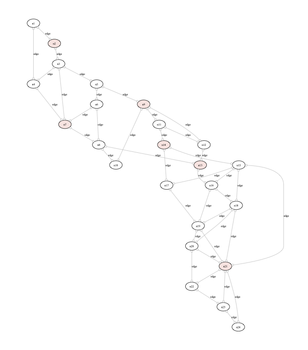
Here is the graphical rendering of a solution using the custom graph definition above:

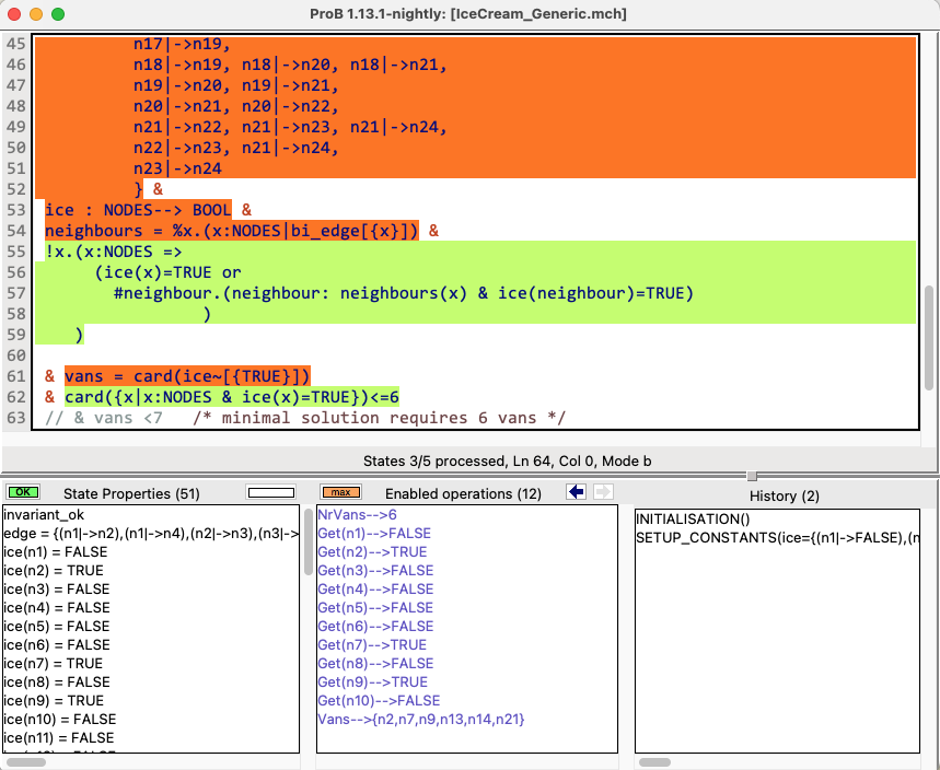
By choosing "Show Source Code Coverage" in the Debug menu of ProB Tcl/Tk you can see which parts of the properties were translated to SAT (in green) and which were processed entirely by ProB (in red-orange):

On the console you can also see feedback about which parts were translated and which ones not.
B2SAT in Jupyter Notebooks
The solve command in the https://gitlab.cs.uni-duesseldorf.de/general/stups/prob2-jupyter-kernel ProB Jupyter kernel now supports sat and satz3 as solvers. They use B2SAT with Glucose and Z3 as SAT solvers respectively.
Here is a simple example to solve a constraint:

This shows how you can use cardinality constraints to iteratively find a minimal dominating set D of a graph g:


