Mutual Exclusion (Fairness)

Consider an Event-B model formalizing an algorithm for mutual exclusion with semaphores for two concurrent processes ${\displaystyle P_{1}}$ and ${\displaystyle P_{2}}$. Each process has been simplified to perform three types of events: request (for entering in the critical section), enter (entering the critical section), and release (exiting the critical section). (For more information on the algorithm and the design of the model see ^[1]).

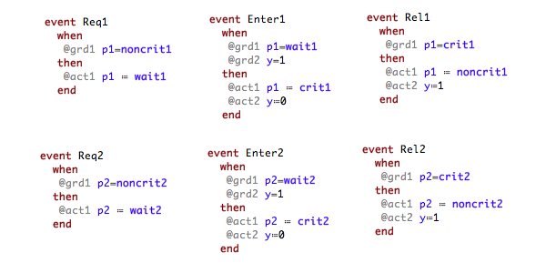
Each of the actions of a process are represented by a respective event:

Each process ${\displaystyle P_{i}}$ has three possible states that are denoted by the constants ${\displaystyle noncrit_{i}}$ (the state in which ${\displaystyle P_{i}}$ performs noncritical actions), ${\displaystyle wait_{i}}$ (the state in which ${\displaystyle P_{i}}$ waits to enter the critical section), and ${\displaystyle crit_{i}}$ (representing the state in which ${\displaystyle P_{i}}$ is in the critical section). Both processes share the binary semaphore y where y=1 indicates that the semaphore is free and y=0 that the semaphore is currently processed by one of the processes.

There are several requirements that the mutual exclusion algorithm should satisfy. The most important one is the mutual exclusion property that says always at most one process is in its critical section. This can be simply expressed, for example, as an invariant of the respective Event-B model: not(p1 = crit1 & p2 = crit2). However, there are other properties that can be easily expressed by means of LTL formulas and automatically checked on the model. For example, the requirement each process will enter infinitely often its critical section can be specified by the LTL formula `GF {p1 = crit1} & GF {p2 = crit2}` or the starvation freedom property that states each waiting process will eventually enter its critical section:

G ({p1 = wait1} => F {p1 = crit1}) & G ({p2 = wait2} => F {p2=crit2}) 

Running the LTL model checker of ProB will provide for the last two properties above a counterexample since the model permits that a process may perform infinitely often consecutively the events request, enter and release, and in this way to ignore the other process infinitely. An example trace that describes this behavior could be ${\displaystyle \langle Req2,Req1,Enter1,Rel1,Req1,Enter1,\ldots \rangle }$.

On the other hand, such behaviors can be considered as unrealistic computations for the eventual implementation of the algorithm. Therefore fairness constraints can be set in order to discard such behaviors. For example, checking the property process ${\displaystyle P_{1}}$ will enter its critical section infinitely often (as LTL property: `GF {p1 = crit1}`) can be checked by restricting that the event `Req1` will not be continuously ignored and that the event `Enter1` will not be ignored infinitely often. Both conditions for the property can be given by means of an LTL^[e] formula on the left side of the following implication:

(FG e(Req1) => GF [Req1]) & (GF e(Enter1) => GF [Enter1]) => GF {p1 = crit1} 

For checking the formula the LTL model checker generates 13312 atoms^[2] and 7515 transitions and needs overall 509 ms to prove the property (the model has 8 states and 15 transitions in total). On the other hand, using the extension of the LTL model checker for checking fairness (by entering the formula `WF(Req1) & SF(Enter1) => GF {p1=crit1}`), the model checker generates 32 atoms and 39 transitions (the atoms and transitions generated just for `GF {p1 = crit1}`) and an overall time of 50 ms.

For checking the requirement each process will enter infinitely often its critical section the LTL formula ` GF {p1 = crit1} & GF {p2 = crit2}` should be checked with the following fairness constraints:

(WF(Req1) & WF(Req2)) & (SF(Enter1) & SF(Enter2))

Encoding these fairness conditions as an LTL^[e] formula will blow up exponentially the number of atoms and the transitions in regard to the number of temporal operators (in this case `G` (globally) and `F`(finally)) and thus make practically impossible to check the above property in a reasonable time.

References