The graphical visualisation of ProB ^[1] enables to easily write custom graphical state representations in order to provide a better understanding of a model. With this method, one assembles a series of pictures and writes an animation function in B. Each picture can be associated to a specific state of a B specification. Then, depending on the current state of the model, the animation function in B stipulates which pictures should be displayed. We now show how this animation can be done with very little effort.

The Graphical Animation Model

The animation model is very simple. It is based on individual images and a user-defined animation function, which are both defined in the DEFINITIONS section of the animated machine as follows:

1. Each image is given a number and its source file location by using the following definition: ANIMATION_IMGx == "filename", where x is the number of the image and "filename" is its path to a gif image file.

2. A user-defined animation function f,,a,, is evaluated to recompute the graphical output for every state. The graphical output of f,,a,, is known as the graphical visualisation, which consists of a two-dimensional grid and where each cell in the grid can contain an image. Depending on row r and column c, an image is displayed in a cell. An image can appear multiple times in the grid.

The function f,,a,, is declared by defining ANIMATION_FUNCTION and must be of type INTEGER * INTEGER +-> INTEGER. If the function f,,a,, is defined for r and c, then the animator should display the image with number f,,a,,(r,c) at row r and column c. Otherwise, no image is displayed in the corresponding cell.

The dimension of the grid is computed by looking at the minimum and maximum coordinates that occur in the animation function. More precisely,

the rows are in the range min(dom(dom(f,,a,,)))..max(dom(dom(f,,a,,))) and

the columns are in the range min(ran(dom(f,,a,,)))..max(ran(dom(f,,a,,))).

We take the B machine of the sliding 8-puzzle as an example. In the 8-puzzle, the tiles are numbered. Every tile can be moved horizontally and vertically into an empty square. The final configuration is reached whenever all the tiles are in order.

The B machine of the 8-puzzle is as follows:

MACHINE Puzzle8
DEFINITIONS INV == (board: ((1..dim)*(1..dim)) -->> 0..nmax);
GOAL == !(i,j).(i:1..dim & j:1..dim => board(i|->j) = j-1+(i-1)*dim);
CONSTANTS dim, nmax
PROPERTIES dim:NATURAL1 & dim=3 & nmax:NATURAL1 & nmax = dim*dim-1
VARIABLES board
INVARIANT INV
INITIALISATION board : (INV & GOAL)
OPERATIONS
 MoveDown(i,j,x) = PRE i:2..dim & j:1..dim & 
                       board(i|->j) = 0 & x:1..nmax & board(i-1|->j) = x
                   THEN board := board <+ {(i|->j)|->x, (i-1|->j)|->0}
                   END;
 MoveUp(i,j,x) = PRE i:1..dim-1 & j:1..dim &
                          board(i|->j) = 0 & x:1..nmax & board(i+1|->j) = x
                 THEN board := board <+ {(i|->j)|->x, (i+1|->j)|->0}
                 END;
 MoveRight(i,j,x) = PRE i:1..dim & j:2..dim &
                        board(i|->j) = 0 & x:1..nmax & board(i|->j-1) = x
                    THEN board := board <+ {(i|->j)|->x, (i|->j-1)|->0}
                    END;
 MoveLeft(i,j,x) = PRE i:1..dim & j:1..dim-1 &
                       board(i|->j) = 0 & x:1..nmax & board(i|->j+1) = x
                   THEN board := board <+ {(i|->j)|->x, (i|->j+1)|->0}
                   END
END

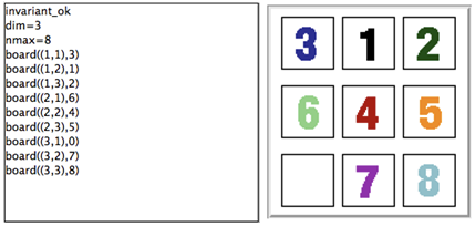
On the left side of the following Figure, the non-graphical visualisation is generated by ProB. It is readable, but the graphical visualisation at the right side is much more inspiring and understandable.

The graphical visualisation is achieved, with very little effort, by writing, in the DEFINITIONS section, the following animation function, as well as the image declaration list:

ANIMATION_FUNCTION == ( {r,c,i|r:1..dim & c:1..dim & i=0} <+ board);
ANIMATION_IMG0 == "images/sm_empty_box.gif"; /* empty square */
ANIMATION_IMG1 == "images/sm_1.gif"; /* square with 1 inside */
ANIMATION_IMG2 == "images/sm_2.gif";
ANIMATION_IMG3 == "images/sm_3.gif";
ANIMATION_IMG4 == "images/sm_4.gif";
ANIMATION_IMG5 == "images/sm_5.gif";
ANIMATION_IMG6 == "images/sm_6.gif";
ANIMATION_IMG7 == "images/sm_7.gif";
ANIMATION_IMG8 == "images/sm_8.gif"; /* square with lightblue 8 inside */

Each of the three integer types in the signature can be replaced by a deferred or enumerated set, in which case our tool translates elements of this set into numbers. In case of enumerated sets, the number is position of the element in the definition of the set in the SETS clause. Deferred set elements are numbered internally by ProB, and this number is used. (Note, however, that the whole animation function has to be of the same type; otherwise the animator will complain about a type error.) To avoid having to produce images for simple strings, one can use a declaration ANIMATION_STRx == "my string" to define image with number x to be automatically generated from the given string.

Typical patterns for the animation function are as follows:

• A useful way to obtain a function of the required signature is to write a set comprehension of the following form:

{row,col,img | row:1..NrRow & col:1..NrCols & P}, 
 where P is a predicate which gives img a value depending on row and col.

• Another useful pattern is to write one function for default images, and then use the override operator to replace the default images only when needed:

DefaultImages <+ CurrentImages

This was used in the 8-Puzzle, by setting as default the empty square (image 0) overriden by the partially defined board function.

• or to write multiple definitions of the animation function. More clearly, we define one animation function for default images and another one for current images as follows:

ANIMATION_FUNCTION_DEFAULT == DefaultImages;
ANIMATION_FUNCTION == CurrentImages;

This was used next in the Sudoku example.

• Translation Predicates between user sets and numbers (extension above can directly handle user sets, but does not work well if we need a special image for undefined,...)

Further Examples

Below we illustrate how the graphical animation model easily provides interesting animations for different models.

Scheduler

The scheduler specification taken from ^[2] is as follows:

MACHINE scheduler
SETS PID = {process1,process2,process3}
VARIABLES active, ready, waiting
INVARIANT active <: PID & ready <: PID & waiting <: PID &
          (ready /\ waiting) = {} & active /\ (ready \/ waiting) = {} &
          card(active) <= 1 & ((active = {}) => (ready = {}))
INITIALISATION active := {} || ready := {} || waiting := {}
OPERATIONS
 new(pp) =
  SELECT pp : PID & pp /: active & pp /: (ready \/ waiting)
  THEN waiting := (waiting \/ { pp })
  END;
 del(pp) =
  SELECT pp : waiting
  THEN waiting := waiting - { pp }
  END;
 ready(rr) = 
  SELECT rr : waiting
  THEN waiting := (waiting - {rr}) ||
       IF (active = {})
       THEN active := {rr}
       ELSE ready := ready \/ {rr} 
       END
  END;
 swap = 
  SELECT active /= {}
  THEN waiting := (waiting \/ active) ||
       IF (ready = {}) THEN active := {}
       ELSE 
        ANY pp WHERE pp : ready
        THEN active := {pp} || ready := ready - {pp}
        END
       END
  END
END

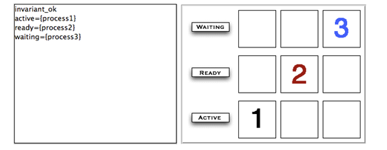
The left side of the following Figure shows the non-graphical animation of the machine scheduler and the right side its graphical animation obtained using ProB.

The graphical visualisation is done by writing, in the DEFINTIONS section, the following animation function. Here, we need to map PID elements to image numbers.

IsPidNrci == p=process1 & i=1) or (p=process2 & i=2) or (p=process3 & i=3));
ANIMATION_FUNCTION == 
 ({1|->0|->5, 2|->0|->6, 3|->0|->7} \/ {r,c,img|r:1..3 & img=4 & c:1..3} <+
 ({r,c,i| r=1 & i:INTEGER & c=i & #p.(p:waiting & IsPidNrci)} \/
 {r,c,i| r=2 & i:INTEGER & c=i & #p.(p:ready & IsPidNrci)} \/
 {r,c,i| r=3 & i:INTEGER & c=i & #p.(p:active & IsPidNrci)} ));
ANIMATION_IMG1 == "images/1.gif";
ANIMATION_IMG2 == "images/2.gif";
ANIMATION_IMG3 == "images/3.gif";
ANIMATION_IMG4 == "images/empty_box.gif";
ANIMATION_IMG5 == "images/Waiting.gif";
ANIMATION_IMG6 == "images/Ready.gif";
ANIMATION_IMG7 == "images/Active.gif"

The previous animation function of scheduler can also be rewritten as follows:

ANIMATION_FUNCTION_DEFAULT ==
 ( {1|->0|->5, 2|->0|->6, 3|->0|->7} \/ {r,c,img|r:1..3 & img=4 & c:1..3} );
ANIMATION_FUNCTION == ({r,c,i| r=1 & i:PID & c=i & i:waiting} \/
                       {r,c,i| r=2 & i:PID & c=i & i:ready} \/
                       {r,c,i| r=3 & i:PID & c=i & i:active}
                      );

Sudoku

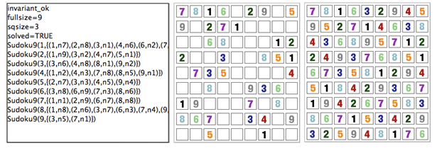
Using ProB, we can also solve Sudoku puzzles. The machine has the variable Sudoku9 of type 1..fullsize-->(1..fullsize+->NRS), where NRS is an enumerate set {n1, n2, ...} of cardinality fullsize.

The animation function is as follows:

Nri == ((Sudoku9(r)(c)=n1 => i=1) & (Sudoku9(r)(c)=n2 => i=2) &
        (Sudoku9(r)(c)=n3 => i=3) & (Sudoku9(r)(c)=n4 => i=4) &
        (Sudoku9(r)(c)=n5 => i=5) & (Sudoku9(r)(c)=n6 => i=6) &
        (Sudoku9(r)(c)=n7 => i=7) & (Sudoku9(r)(c)=n8 => i=8) &
        (Sudoku9(r)(c)=n9 => i=9) 
       );
ANIMATION_FUNCTION == ({r,c,i|r:1..fullsize & c:1..fullsize & i=0} <+
                       {r,c,i|r:1..fullsize & c:1..fullsize &
                       c:dom(Sudoku9(r)) & i:1.. fullsize & Nri}
                      );

The following Figure shows the non-graphical visualisation of a particular puzzle (left), then the graphical visualisation of the puzzle (middle), as well as the visualisation of the solution found by ProB after a couple of seconds (right).

Note that it would have been nice to be able to replace Nri inside the animation function simply by i = Sudoku9(r)(c). While our visualisation algorithm can automatically convert set elements to numbers, the problem is that there is a type error in the override: the left-hand side is a function of type INTEGER*INTEGER+->INTEGER while the right-hand side now becomes a function of type INTEGER*INTEGER+->NRS. One solution is to write multiple definitions of the animation function. In addition to the standard animation function, we can define a default background animation function. The standard animation function will override the default animation function, but the overriding is done within the graphical animator and not within a B formula. In this way, one can now rewrite the above animation as follows:

ANIMATION_FUNCTION_DEFAULT == ( {r,c,i|r:1..fullsize & c:1..fullsize & i=0} );
ANIMATION_FUNCTION == ({r,c,i|r:1..fullsize & c:1..fullsize &
                       c:dom(Sudoku9(r)) & i:1.. fullsize & i = Sudoku9(r)(c)}
                      )

References

- ↑ M. Leuschel, M. Samia, J. Bendisposto and L. Luo: Easy Graphical Animation and Formula Viewing for Teaching B. In C. Attiogbé and H. Habrias, editors, Proceedings: The B Method: from Research to Teaching, pages 17-32, Nantes, France. APCB, 2008.
- ↑ B. Legeard, F. Peureux, and M. Utting. Automated boundary testing from Z and B. Proceedings of FME’02, LNCS 2391, pages 21–40. Springer-Verlag, 2002.