The current versions of ProB can make use of the new B2SAT backend as an alternate way of solving constraints. It translates a subset of B formulas to SAT and for solving by an external SAT solver. The new backend interleaves low-level SAT solving with high-level constraint solving performed by the default solver of ProB.

B2SAT solving consists of the following phases:

• the deterministic propagation phase(s) of ProB's solver: it performs deterministic propagations and can expand quantifiers and total functions.
• a compilation phase, whereby static values are inlined.
• the B to CNF conversion proper, which can translate a subset of B to propositional logic in conjunctive normal form. This phase currently supports:
  • equalities and inequalities between boolean variables and constants,
  • all logical connectives and
  • some cardinality constraints.
  • Subformulas that cannot be solved are sent to ProB's default solver and linked to the CNF via an auxiliary propositional variable.
• solving phase, where the generated CNF is sent to an external SAT solver.
• propagation of the SAT solution to B, by progressively grounding the B values and predicates linked to the propositional variables.
• complete constraint solving, solving the pending constraints in B by now performing the regular non-deterministic propagations and enumerations of ProB.

Using B2SAT

B2SAT in the REPL

The following four commands are now available in REPL of probcli (start with probcli --repl):

• :sat PRED
• :sat-z3 PRED
• :sat-double-check PRED
• :sat-z3-double-check PRED

Here is a simple example:

 >>> :sat f:1..n --> BOOL & n=3 & f(1)=TRUE & !i.(i:2..n => f(i) /= f(i-1))
 PREDICATE is TRUE
 Solution: 
        f = {(1|->TRUE),(2|->FALSE),(3|->TRUE)} &
        n = 3

B2SAT for PROPERTIES

The new preference SOLVER_FOR_PROPERTIES can be used to specify solver for PROPERTIES (axioms) when setting up constants. The valid settings are: prob (the default), kodkod, z3, z3cns, z3axm, cdclt, sat, sat-z3.

The last two will use B2SAT, sat with Glucose as SAT solver and sat-z3 with Z3 as SAT solver.

Here is an example using this preference to compute a dominating set of a graph:

MACHINE IceCream_Generic
// Dominating set example:
// place ice cream vans so that every house (node) is at most one block away from a van
DEFINITIONS
  N == 24;
  CUSTOM_GRAPH == rec(layout:"dot", rankdir:"TB",
                     nodes: {j•j:NODES |
                               rec(value:j, style:"filled",
                                fillcolor:IF ice(j)=TRUE THEN "mistyrose" ELSE "white" END
                                  )},
                    edges:rec(color:"gray", arrowhead:"odot",
                              arrowtail:"odot", dir:"both",
                              label:"edge",   edges: edge)
                    );
      bi_edge == (edge \/ edge~);
  SET_PREF_SOLVER_FOR_PROPERTIES == "sat";
SETS
  NODES = {n1,n2,n3,n4,n5,n6,n7,n8,n9,n10,
           n11,n12,n13,n14,n15,n16,n17,n18,n19,n20,n21,n22,n23,n24}
CONSTANTS edge, ice, vans, neighbours
PROPERTIES
 edge: NODES <-> NODES &
 edge = { n1|->n2, n1|->n4,
          n2|->n3,
          n3|->n4, n3|->n5, n3|->n7,
          n4|->n7,
          n5|->n6, n5|->n9,
          n6|->n7, n6|->n8,
          n7|->n8,
          n8|->n10, n8|->n13,
          n9|->n10, n9|->n11, n9|->n12,
          n11|->n12, n11|->n14,
          n12|->n13,
          n13|->n16,
          n14|->n15, n14|->n17,
          n15|->n16, n15|->n17, n15|->n18, n15|->n21,
          n16|->n18, n16|->n19,
          n17|->n19,
          n18|->n19, n18|->n20, n18|->n21,
          n19|->n20, n19|->n21,
          n20|->n21, n20|->n22,
          n21|->n22, n21|->n23, n21|->n24,
          n22|->n23, n21|->n24,
          n23|->n24
          } &
 ice : NODES--> BOOL &
 neighbours = %x.(x:NODES|bi_edge[{x}]) &
 !x.(x:NODES =>
      (ice(x)=TRUE or
        #neighbour.(neighbour: neighbours(x) & ice(neighbour)=TRUE)
                 )
    )
 & vans = card(ice~[{TRUE}])
 & card({x|x:NODES & ice(x)=TRUE})<=6  /* minimal solution requires 6 vans */
OPERATIONS
  v <-- NrVans = BEGIN v := vans END;
  xx <-- Get(yy) = PRE yy:NODES THEN xx:= ice(yy) END;
  v <-- Vans = BEGIN v:= ice~[{TRUE}] END
END

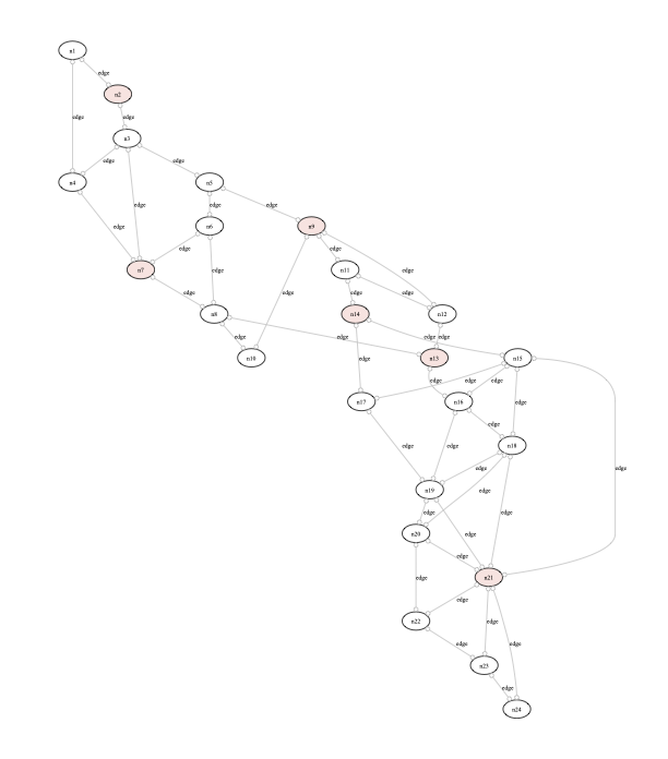
Here is the graphical rendering of a solution using the custom graph definition above:

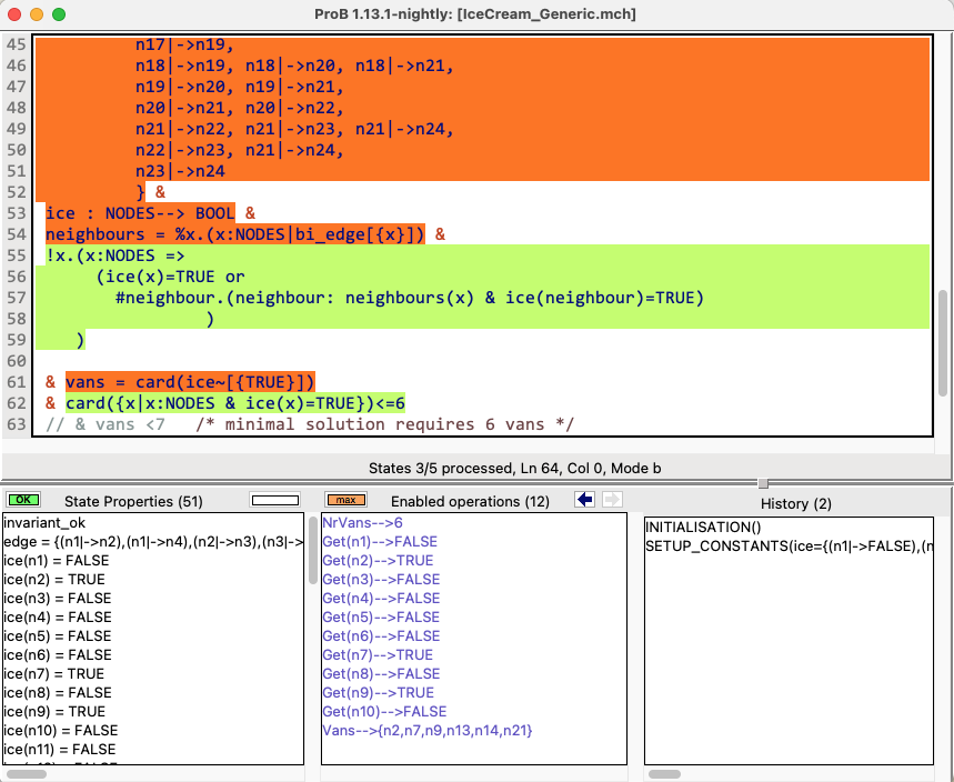
By choosing "Show Source Code Coverage" in the Debug menu of ProB Tcl/Tk you can see which parts of the properties were translated to SAT (in green) and which were processed entirely by ProB (in red-orange):

On the console you can also see feedback about which parts were translated and which ones not.

B2SAT in Jupyter Notebooks

The solve command in the ProB Jupyter kernel now supports sat and satz3 as solvers. They use B2SAT with Glucose and Z3 as SAT solvers respectively.

Here is a simple example to solve a constraint:

This shows how you can use cardinality constraints to iteratively find a minimal dominating set D of a graph g:

B2SAT for TLA+, Z and Alloy

B2SAT is also available for other state-based languages supported by ProB.

Below is the dominating set example from above as a TLA+ machine that can be loaded and solved by ProB. The custom graph visualisation derived from CUSTOM_GRAPH is also similar.

---- MODULE IceCream_Generic_cst ----
EXTENDS Naturals, FiniteSets
CONSTANTS n1, n2, n3, n4, n5, n6, n7, n8, n9, n10, 
          n11, n12, n13, n14, n15, n16, n17, n18, n19, n20,
          n21, n22, n23, n24,
          ice
VARIABLES vans
NODES == {n1, n2, n3, n4, n5, n6, n7, n8, n9, n10, n11, n12, n13, n14, n15, n16, n17, n18, n19, n20, n21, n22, n23, n24}

SET_PREF_TIME_OUT == 1500
SET_PREF_SOLVER_FOR_PROPERTIES == "sat"

edge == {<<n1, n2>>, <<n1, n4>>, <<n2, n3>>, <<n3, n4>>, <<n3, n5>>, <<n3, n7>>, <<n4, n7>>, <<n5, n6>>, <<n5, n9>>, <<n6, n7>>, <<n6, n8>>, <<n7, n8>>, <<n8, n10>>, <<n8, n13>>, <<n9, n10>>, <<n9, n11>>, <<n9, n12>>, <<n11, n12>>, <<n11, n14>>, <<n12, n13>>, <<n13, n16>>, <<n14, n15>>, <<n14, n17>>, <<n15, n16>>, <<n15, n17>>, <<n15, n18>>, <<n15, n21>>, <<n16, n18>>, <<n16, n19>>, <<n17, n19>>, <<n18, n19>>, <<n18, n20>>, <<n18, n21>>, <<n19, n20>>, <<n19, n21>>, <<n20, n21>>, <<n20, n22>>, <<n21, n22>>, <<n21, n23>>, <<n21, n24>>, <<n22, n23>>, <<n21, n24>>, <<n23, n24>>}

DomSet == (\A x \in NODES : (ice[x] = TRUE \/ (\E nbour \in NODES : (<<nbour,x>> \in edge \/ <<x,nbour>> \in edge) /\ ice[nbour] = TRUE)))

ASSUME ice \in [NODES -> BOOLEAN] /\ DomSet /\ Cardinality({x \in (NODES): ice[x] = TRUE}) =< 6

Init == 
	vans = Cardinality({x\in NODES : ice[x]=TRUE})

Invariant == 
	vans \in (0 .. 10)

Next == UNCHANGED <<ice, vans>>

CUSTOM_GRAPH == [layout |-> "dot", rankdir |-> "TB", 
  nodes |-> {[value |-> j, style |-> "filled", 
              fillcolor |-> (IF ice[j] = TRUE THEN "mistyrose" ELSE "white")]: j \in NODES}, 
  edges |-> [color |-> "gray", arrowhead |-> "odot", arrowtail |-> "odot", dir |-> "both", label |-> "edge",
             edges |-> edge]]
====