SimB: Difference between revisions
| Line 205: | Line 205: | ||
The operations' substitutions model the desired behavior of the respective actions. | The operations' substitutions model the desired behavior of the respective actions. | ||
An example for the FASTER of a HighwayEnvironment is as follows: | |||
<pre> | |||
FASTER = | |||
PRE | |||
¬(∃v. (v ∈ PresentVehicles \ {EgoVehicle} ∧ VehiclesX(v) > 0.0 ∧ VehiclesX(v) < 45.0 ∧ | |||
VehiclesY(v) < 3.5 ∧ VehiclesY(v) > -3.5)) | |||
THEN | |||
Crash :∈ BOOL || | |||
PresentVehicles :∈ P(Vehicles) ; | |||
VehiclesX :∈ Vehicles → R || | |||
VehiclesY :∈ Vehicles → R || | |||
VehiclesVx :| (VehiclesVx ∈ PresentVehicles → R ∧ | |||
VehiclesVx(EgoVehicle) ≥ | |||
VehiclesVx ’(EgoVehicle) - 0.05) || | |||
VehiclesVy :∈ Vehicles → R || | |||
VehiclesAx :| (VehiclesAx ∈ PresentVehicles → R ∧ | |||
VehiclesAx(EgoVehicle) ≥ -0.05) || VehiclesAy :∈ Vehicles → R || | |||
Reward :∈ R | |||
END | |||
</pre> | |||
2. Implement the mapping between the RL agent in Python and the formal B model | 2. Implement the mapping between the RL agent in Python and the formal B model | ||
Revision as of 20:52, 14 January 2024
SimB
SimB is a simulator built on top of ProB. It is available in the latest SNAPSHOT version in the new JavaFX based user interface ProB2-UI (https://github.com/hhu-stups/prob2_ui), The modeler can write SimB annotations for a formal model to simulate it. Examples are available at https://github.com/favu100/SimB-examples. Furthermore, it is then possible to validate probabilistic and timing properties with statistical validation techniques such as hypothesis testing and estimation.
SimB also contains a feature called interactive simulation. This feature allows user interaction to trigger a simulation. For interactive simulation, a modeler has to encode SimB listeners on events, triggering a SimB simulation. Interactive Simulation examples are available at https://github.com/favu100/SimB-examples/tree/main/Interactive_Examples.
More recently, SimB is extended by a new feature which makes it possible to load an Reinforcement learning Agent.
Technically, each step of the RL agent is converted into a SimB activation.
In order to simulate a RL agent in SimB, one must (1) create a formal B model for the RL agent, and (2) create a mapping between the state in the RL agent and the formal model, and (3) provide information to the formal B model again.
Reinforcement Learning examples are available at: https://github.com/hhu-stups/reinforcement-learning-b-models
Citing SimB
To cite SimB as a tool, its timing or probabilistic simulation features, or SimBs statistical validation techniques, please use:
@InProceedings{simb,
  Author    = {Vu, Fabian and Leuschel, Michael and Mashkoor, Atif},
  Title        = {{Validation of Formal Models by Timed Probabilistic Simulation}},
  Booktitle    = {Proceedings ABZ},
  Year        = 2021,
  Series    = {LNCS},
  Volume     = {12709},
  Pages = {81--96}
}
To cite SimBs interactive simulation, please use:
@InProceedings{simb,
  Author    = {Vu, Fabian and Leuschel, Michael},
  Title        = {{Validation of Formal Models by Interactive Simulation}},
  Booktitle    = {Proceedings ABZ},
  Year        = 2023
  Series = {LNCS},
  Volume = {14010},
  Pages = {59--69}
}
Using SimB
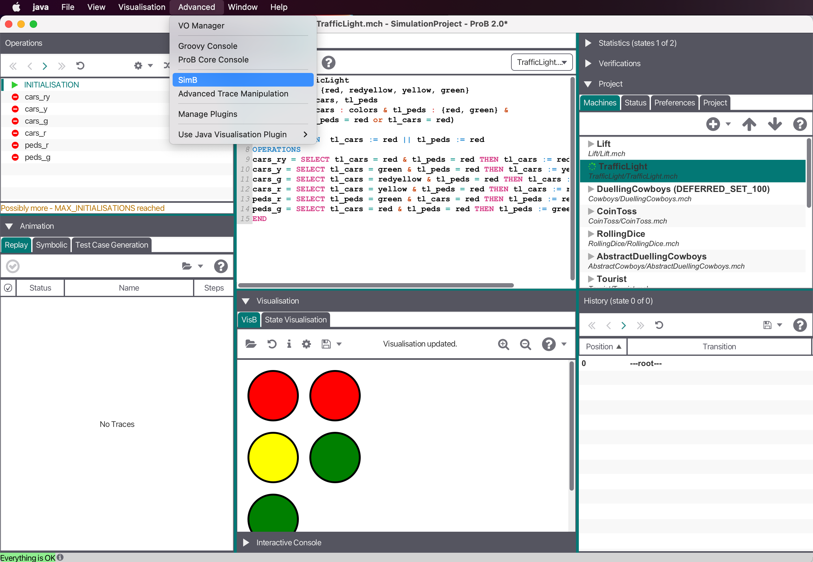
Start SimB via "SimB" in the "Advanced" Menu after opening a machine.
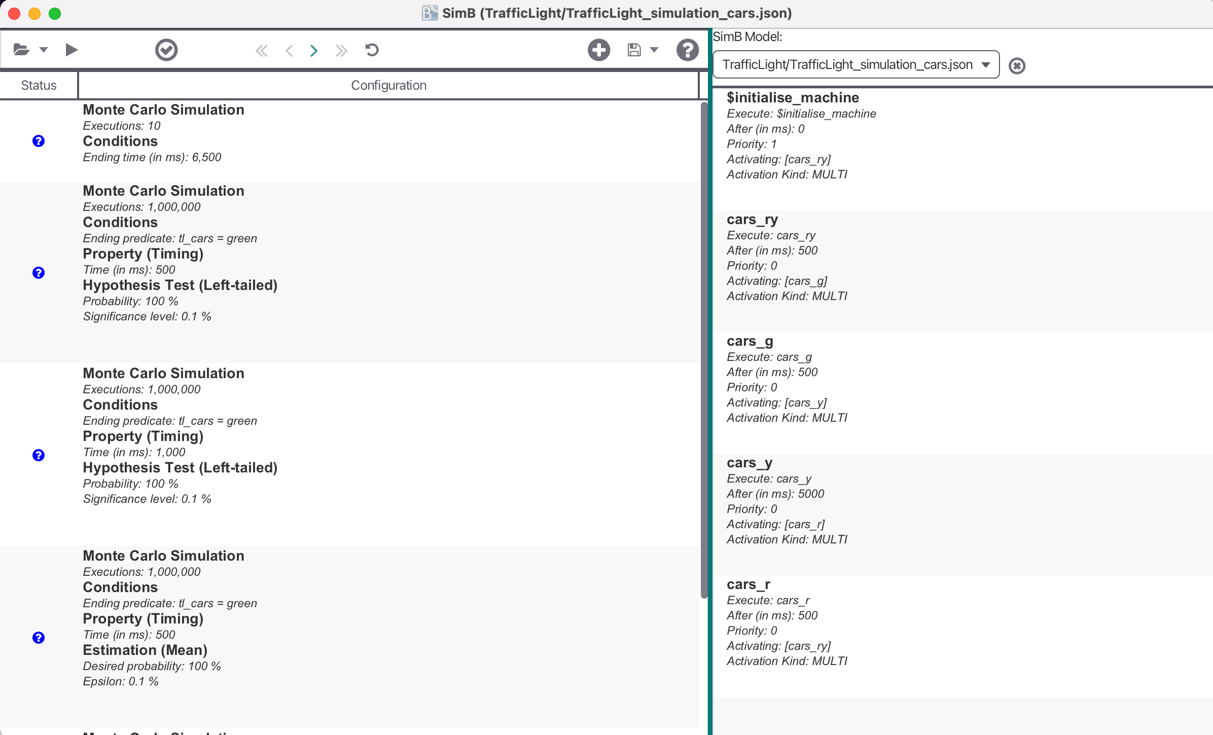
Now, you can open a SimB file (JSON format) controlling the underlying formal model.
A SimB file consists of SimB activations and SimB listeners to simulate the model. SimB activations encode an activation diagram with probabilistic and timing elements for automatic simulation. To enable interactive simulation, it is also necessary to encode interactive elements aka. SimB listeners which trigger other SimB activations. Within these elements, the modeler can user B expressions which are evaluated on the current state.
The general structure of a SimB simulation is as follows:
{
  "activations": [...]
  "listeners": [...]
}
activations stores SimB activations, while listeners stores SimB listeners. activations must be encoded, listeners is optional and defaults to the empty list.
Probabilistic and Timing Elements in SimB
The SimB file always contains an activations field storing a list of probabilistic and timing elements to control the simulation. Probabilistic values are always evaluated to ensure that the sum of all possibilities is always 1. Otherwise an error will be thrown at runtime. There are two types of activations: direct activation and probabilistic choice. All activations are identified by their id.
Direct Activation
A direct activation activates an event to be executed in the future. It requires the fields id, and execute to be defined. All other fields can be defined optionally.
- execute identifies the activated event by its name.
- after defines the scheduled time (in ms) when activating an event. By default, it is set to 0 ms, e.g., when this field is not defined explicitly.
- activating stores events that will be activated when executing the event defined by execute. Missing definition leads to the behavior that no other events are activated. The modeler can either write a String (to activate a single event) or a list of Strings (to activate multiple events)
- activationKind stores the kind of activation for execute. Possible options are multi, single, single:min, and single:max. The default value is multi
- multi means that the activation will be queued for execution.
- single means that the activation will only be queued if there are no queued activations with the same id
- single:min means that the activation will only be queued if (1) there are no queued activations for the same id or (2) there is a queued activation with the same id whose value for the scheduled time is greater. In the case of (2), the already queued activation will be discarded.
- single:max means that the activation will only be queued if (1) there are no queued activations for the same id or (2) there is a queued activation with the same id whose value for the scheduled time is lower. In the case of (2), the already queued activation will be discarded.
- additionalGuards stores optional guards when executing the event stored in execute
- fixedVariables stores a Map. Here, a variable (parameter, or non-deterministic assigned variable) is assigned to its value.
- probabilisticVariables stores either a Map or a String. Concerning the Map, a variable (parameter, or non-deterministic assigned variable) is assigned to another Map defining the probabilistic choice of its value. The second Map stores Key-Value pairs where values are mapped to the probability. The modeler can also assign probabilisticVariables to first or uniform.
- first means that the first transition is chosen for execution.
- uniform means that a transition is selected from all alternatives uniformly.
- priority stores the priority for scheduling execute. Lower number means greater priority.
{
   "id":  ...
   "execute": ...
   "after": ...
   "activating": ...
   "activationKind": ...
   "additionalGuards": ...
   "fixedVariables": ....
   "probabilisticVariables": ....
   "priority": ...
}
Probabilistic Choice
A probabilistic choice selects an event to be executed in the future. It requires the two fields id, and chooseActivation. chooseActivation is a Map storing Key-Value pairs where activations (identified by their id) are mapped to a probability. It is possible to chain multiple probabilistic choices together, but eventually, a direct activation must be reached.
{
   "id":  ...
   "chooseActivation": ...
}
In the following, an example for a SimB file controlling a Traffic Lights for cars and pedestrians (with timing and probabilistic behavior) is shown:
{
 "activations": [
  {"id":"$initialise_machine", "execute":"$initialise_machine", "activating":"choose"},
  {"id":"choose", "chooseActivation":{"cars_ry": "0.8", "peds_g": "0.2"}},
  {"id":"cars_ry", "execute":"cars_ry", "after":5000, "activating":"cars_g"},
  {"id":"cars_g", "execute":"cars_g", "after":500, "activating":"cars_y"},
  {"id":"cars_y", "execute":"cars_y", "after":5000, "activating":"cars_r"},
  {"id":"cars_r", "execute":"cars_r", "after":500, "activating":"choose"},
  {"id":"peds_g", "execute":"peds_g", "after":5000, "activating":"peds_r"},
  {"id":"peds_r", "execute":"peds_r", "after":5000, "activating":"choose"}
 ]
}
Interactive Elements in SimB
Interactive elements in SimB are so called SimB listeners. A SimB listener consists of four fields id, event, predicate, and activating. This means that the SimB listener associated with id listens on a manual/user interaction on event with predicate after which activations in activating are triggered. predicate is optional and defaults to 1=1. Manual/User interaction is recognized via VisB and ProB's Operations View.
{
   "id":  ...
   "event": ...
   "predicate": ...
   "activating": [...]
}
In the following, we parts of a SimB simulation from an automotive case study. The SimB simulation contains a SimB listener which is linked to two activations. The case study models the car's lighting system controlled by pitman controller, the key ignition, and the warning lights button.
The SimB listeners states that SimB listens on user interaction on the event ENV_Pitman_DirectionBlinking, to trigger two SimB activations blinking_on and blinking_off afterward. Practically, this means that a driver's input on the pitman for direction blinking activates the blinking cycle for the corresponding direction indicators.
{
  "activations": [
    {
      "id": "blinking_on",
      "execute": "RTIME_BlinkerOn",
      "after": "curDeadlines(blink_deadline)",
       "activating" : "blinking_off",
       ...
    },
    {
      "id": "blinking_off",
      "execute": "RTIME_BlinkerOff",
      "after": "curDeadlines(blink_deadline)",
       "activating" : "blinking_on",
       ...
    },
    ...
  ]
  "listeners": [
    {
      "id": "start_blinking",
      "event": "ENV_Pitman_DirectionBlinking",
      "activating" : ["blinking_on", "blinking_off"]
    }
  ]
}
Reinforcement Learning Agent in SimB
Instead of loading a SimB simulation as a JSON file, one can also load a Reinforcement Learning agent implemented in Python (.py). For the simulation to work, one has to apply the following steps:
1. Create a formal B model (including safety shield).
The operations represent the actions the RL agent can choose from. The formal model's state mainly represents the state of the environment. Safety shields are encoded by the operations' guards which are provided to the RL agent. Enabled operations are considered to be safe. Thus, the RL agent chooses the enabled operation/action with the highest predicted reward. The operations' substitutions model the desired behavior of the respective actions.
An example for the FASTER of a HighwayEnvironment is as follows:
FASTER =
PRE
  ¬(∃v. (v ∈ PresentVehicles \ {EgoVehicle} ∧ VehiclesX(v) > 0.0 ∧ VehiclesX(v) < 45.0 ∧
  VehiclesY(v) < 3.5 ∧ VehiclesY(v) > -3.5))
THEN
  Crash :∈ BOOL ||
  PresentVehicles :∈ P(Vehicles) ;
  VehiclesX :∈ Vehicles → R ||
  VehiclesY :∈ Vehicles → R ||
  VehiclesVx :| (VehiclesVx ∈ PresentVehicles → R ∧
  VehiclesVx(EgoVehicle) ≥
  VehiclesVx ’(EgoVehicle) - 0.05) ||
  VehiclesVy :∈ Vehicles → R ||
  VehiclesAx :| (VehiclesAx ∈ PresentVehicles → R ∧
  VehiclesAx(EgoVehicle) ≥ -0.05) || VehiclesAy :∈ Vehicles → R ||
  Reward :∈ R
END
2. Implement the mapping between the RL agent in Python and the formal B model
3. Implement necessary messages sent between the ProB animator and the RL agent. Simulation should be a while-loop which runs while the simulation has not finished.
- 1st message: Sent from ProB Animator: List of enabled operations
- Meanwhile RL agent predicts enabled operation with highest reward
- 2nd message: Sent from RL agent: Name of chosen action/operation
- 3rd message: Sent from RL agent: Time until executing chosen action/operation
- 4th message: Sent from RL agent: Succeeding B state as a predicate
- 5th message: Sent from RL agent: Boolean flag describing whether simulation is finished
Example code (line 70 - 113; particularly 86 - 113): https://github.com/hhu-stups/reinforcement-learning-b-models/blob/main/HighwayEnvironment/HighwayEnvironment.py
Validation
Real-Time Simulation
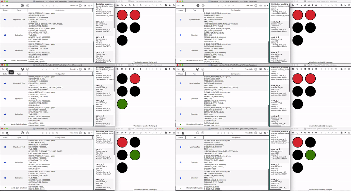
Using a SimB file, the modeler can play a single simulation on the underlying model in real-time. The modeler can then manually check whether the model behaves as desired. Combining VisB and SimB, a simulation can be seen as an animated picture similar to a GIF picture. This gives the domain expert even a better understanding of the model. With SimB listeners, it is also possible to encode simulations that are triggered by manual/user actions.
A Traffic Light example (based on the SimB file shown in Using_SimB ) simulating the first 21 seconds is shown below.
Timed Trace Replay
Based on a single simulation, the modeler can generate a timed trace which is also stored in the SimB format. Afterwards, it can be used to replay a scenario. similar to real-time simulation.
Below, the resulting timed trace for the scenario in Real-Time Simulation is shown
{
  "activations": [
    {
      "execute": "$initialise_machine",
      "after": "0",
      "priority": 0,
      "additionalGuards": null,
      "activationKind": null,
      "fixedVariables": {
        "tl_cars": "red",
        "tl_peds": "red"
      },
      "probabilisticVariables": null,
      "activating": [
        "cars_ry_1"
      ],
      "id": "$initialise_machine"
    },
    {
      "execute": "cars_ry",
      "after": "5000",
      "priority": 0,
      "additionalGuards": null,
      "activationKind": null,
      "fixedVariables": null,
      "probabilisticVariables": null,
      "activating": [
        "cars_g_2"
      ],
      "id": "cars_ry_1"
    },
    {
      "execute": "cars_g",
      "after": "500",
      "priority": 0,
      "additionalGuards": null,
      "activationKind": null,
      "fixedVariables": null,
      "probabilisticVariables": null,
      "activating": [
        "cars_y_3"
      ],
      "id": "cars_g_2"
    },
    {
      "execute": "cars_y",
      "after": "5000",
      "priority": 0,
      "additionalGuards": null,
      "activationKind": null,
      "fixedVariables": null,
      "probabilisticVariables": null,
      "activating": [
        "cars_r_4"
      ],
      "id": "cars_y_3"
    },
    {
      "execute": "cars_r",
      "after": "500",
      "priority": 0,
      "additionalGuards": null,
      "activationKind": null,
      "fixedVariables": null,
      "probabilisticVariables": null,
      "activating": [
        "peds_g_5"
      ],
      "id": "cars_r_4"
    },
    {
      "execute": "peds_g",
      "after": "5000",
      "priority": 0,
      "additionalGuards": null,
      "activationKind": null,
      "fixedVariables": null,
      "probabilisticVariables": null,
      "activating": [
        "peds_r_6"
      ],
      "id": "peds_g_5"
    },
    {
      "execute": "peds_r",
      "after": "5000",
      "priority": 0,
      "additionalGuards": null,
      "activationKind": null,
      "fixedVariables": null,
      "probabilisticVariables": null,
      "activating": null,
      "id": "peds_r_6"
    }
  ],
  "metadata": {
    "fileType": "Timed_Trace",
    "formatVersion": 1,
    "savedAt": "2021-03-03T11:04:08.460477Z",
    "creator": "User",
    "proB2KernelVersion": "4.0.0-SNAPSHOT",
    "proBCliVersion": null,
    "modelName": null
  }
}
Monte Carlo Simulation
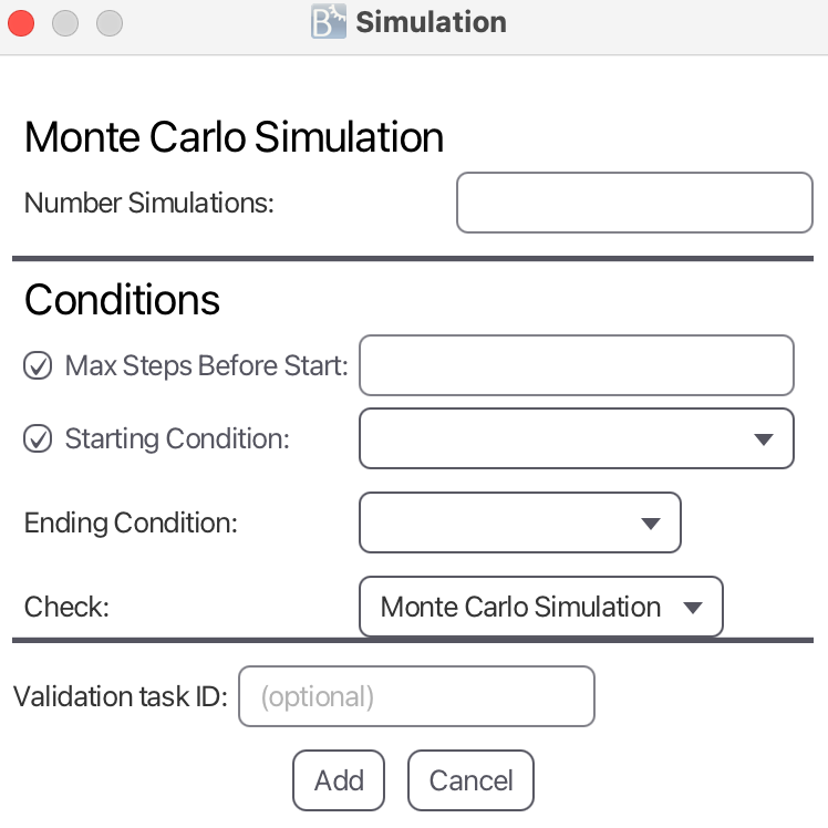
It is also possible to apply Monte Carlo simulation to generate a certain number of simulations. Here, all simulations are played without real time. However, it is possible for the user, to replay the generated scenarios with real-time afterwards.
The input parameters are:
- Number of Simulations defines the number of simulations to be generated.
- Max Steps Before Start defines the number of steps before taking into account the starting and ending conditions.
- Starting Condition defines condition to simulate until before taking Ending Condition into account. It is either defined by a No Condition, Number of Steps, Starting Time or Starting Predicate.
- Ending Condition defines condition to simulate until after taking Starting Condition into account (defines the last transition of the simulation). It is either defined by a Number of Steps, Ending Time or Ending Predicate
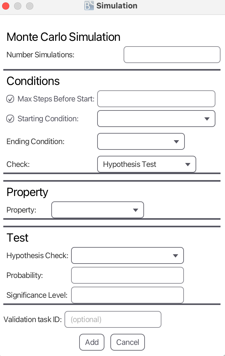
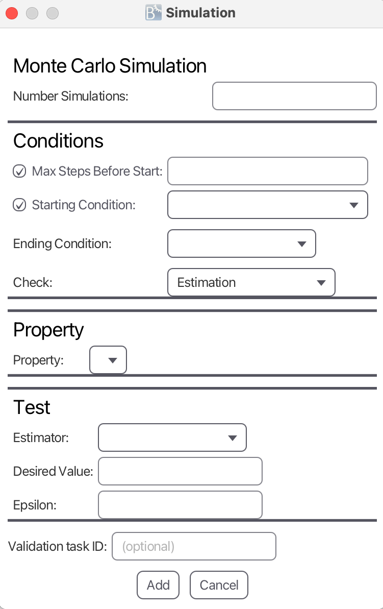
- Check defines the check to apply for the simulation. Monte Carlo Simulation means that there are no checks to be applied, while the other options are Hypothesis Testing and Estimation
Furthermore, there are two statistical validation techniques that can be applied based on Monte Carlo simulations: Hypothesis Testing and Estimation.
Hypothesis Testing
Hypothesis Testing expects the same parameters as Monte Carlo Simulation: Max Steps before Simulation, Number of Simulations, Starting Condition and Ending Condition.
The additional input parameters for Hypothesis Testing are:
- Property defines the property to be checked between Starting Condition and Ending Condition for each simulation. Possible configurations are:
- All Invariants can be used to check all invariants.
- Predicate as Invariant can be used to provide a predicate to be checked whether it is always true.
- Final Predicate can be used to provide a predicate to be checked in the final state of a simulation.
- Predicate Eventually can be used to provide a predicate to be checked whether it is eventually true.
- Timing can be used to check the time.
- Hypothesis Check
- Left-tailed hypothesis test
- Right-tailed hypothesis test
- Two-tailed hypothesis test
- Probability (in the hypothesis)
- Significance Level
Estimation
Estimation expects the same parameters as Monte Carlo Simulation: Number of Simulations, Starting Condition and Ending Condition.
The additional input parameters for Estimation are:
- Property defines the property to be checked between Starting Condition and Ending Condition for each simulation. Possible configurations are:
- All Invariants can be used to check all invariants.
- Predicate as Invariant can be used to provide a predicate to be checked whether it is always true.
- Final Predicate can be used to provide a predicate to be checked in the final state of a simulation.
- Predicate Eventually can be used to provide a predicate to be checked whether it is eventually true.
- Timing can be used to check the time.
- Average can be used to check the average value of an expression.
- Sum can be used to check the sum of an expression.
- Estimator
- Minimum Estimator returns the minimum estimated value from all simulated runs.
- Mean Estimator returns the mean estimated value from all simulated runs.
- Maximum Estimator returns the maximum estimated value from all simulated runs.
- Desired Value
- Epsilon
For an estimated value e, a desired value d, and an epsilon eps, it checks for each simulation whether e is within [d - eps, d + eps]
