Argumentation Theory: Difference between revisions

Below we try to model some concepts of argumentation theory in B. The examples try to show that classical (monotonic) logic with set theory can be used to model some aspects of argumentation theory quite naturally, and that ProB can solve and visualise some problems in argumentation theory. Alternative solutions are encoding arguments as normal logic programs (with non-monotonic negation) and using answer set solvers for problem solving.

The following model was inspired by a talk given by Claudia Schulz.

The model below represents the labelling of the arguments as a total function from arguments to its status, which can either be in (the argument is accepted), out (the argument is rejected), or undec (the argument is undecided). The relation between the arguments is given in the binary attacks relation.

In case you are new to B, you probably need to know the following operators to understand the specification below (we als have a summary page about the B syntax):

• x : S specifies that x is an element of S
• a|->b represents the pair (a,b); note that a relation and function in B is a set of pairs.
• x|->y : R hence specifies that x is mapped to y in relation R
• !x.(P => Q) denotes universal quantification over variable x
• #x.(P & Q) denotes existential quantification over variable x
• A <--> B denotes the set of relations from A to B
• A --> B denotes the set of total functions from A to B
• block comments are of the form /* ... */ and line comments start with // (be sure to use version 1.5.1 of ProB, e.g., from the Nightly download site as line comments were added recently to B)

MACHINE ArgumentationTotFun
SETS
 ARGUMENTS={A,B,C,D,E};
 STATUS = {in,out,undec}
CONSTANTS attacks, label
PROPERTIES
  attacks : ARGUMENTS <-> ARGUMENTS  /* which argument attacks which other argument */
  &
  label: ARGUMENTS --> {in,out,undec} & /* the labeling function */

  // if an argument y is in any attacker must be out:
  !(x,y).(x|->y:attacks => (label(y)=in => label(x)=out)) &
  // if an argument x is in anything it attacks must be out: 
  !(x,y).(x|->y:attacks => (label(x)=in => label(y)=out)) &
  //if an argument y is out it must be attacked by a valid argument:
  !(y).(y:ARGUMENTS => (label(y)=out => #x.(x|->y:attacks & label(x)=in))) & 
  // if an argument y is undecided it must be attacked by an undecided argument:
  !(y).(y:ARGUMENTS => (label(y)=undec => #x.(x|->y:attacks & label(x)=undec))) 
 &
  // here we model one particular argumentation graph
  // A = the sun will shine to day, B = we are in the UK, C = it is summer, D = there are only 10 days of sunshine per year, E = the BBC has forecast sun
  attacks = {B|->A, C|->B, D|->C, E |-> B, E|->D} 
END

Here is a screenshot of ProB Tcl/Tk after loading the model.

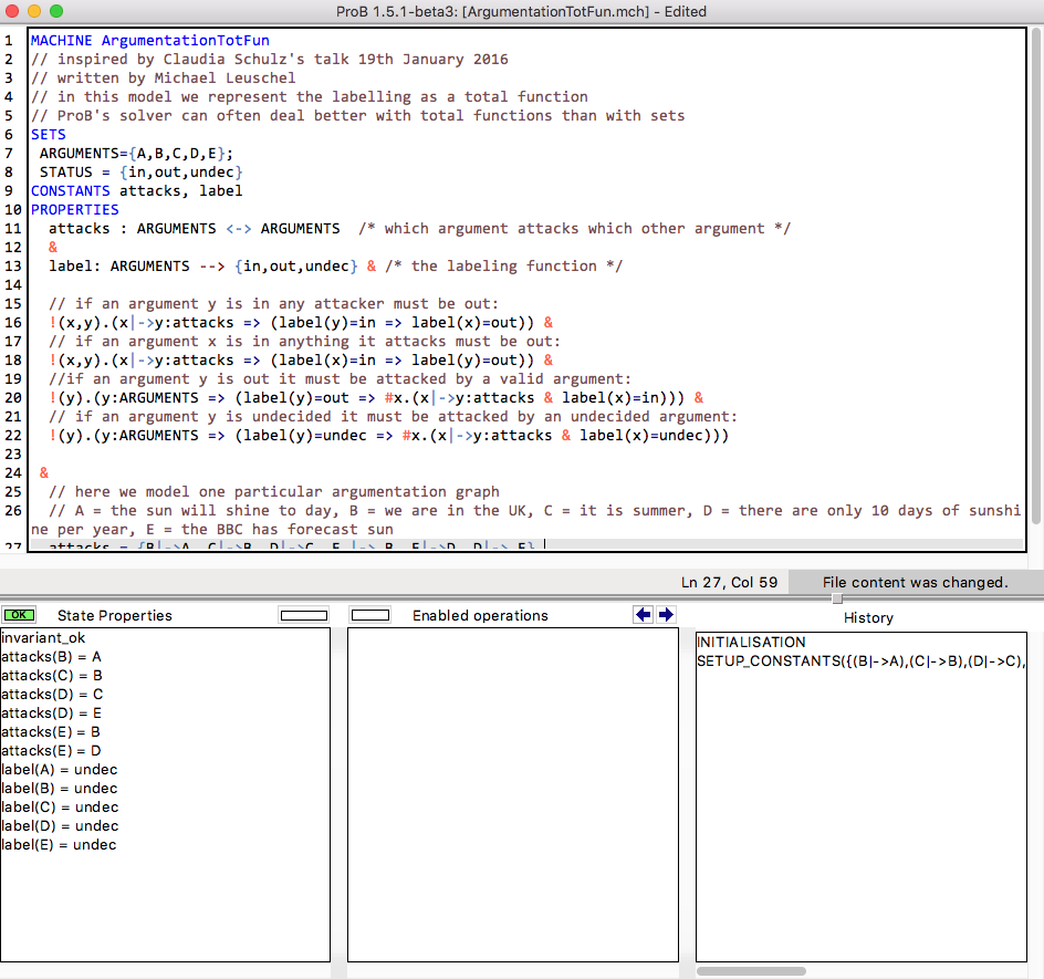
You can see that there is only a single solution (solving time 10 ms), as only a single SETUP_CONSTANTS line is available in the "Enabled Operations" pane. Double-click on SETUP_CONSTANTS and then INITIALISATION will give you the following result, where you can see the solution in the "State Properties" pane:

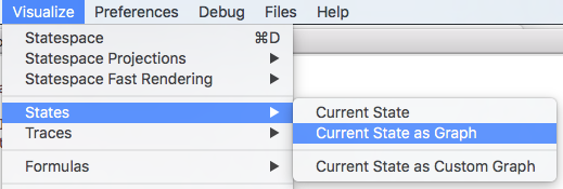
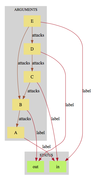
If you want to inspect the solution visually, you can select the "Current State as Graph" command in the "States" submenu of the "Visualize" menu:

This results in the following picture being displayed:

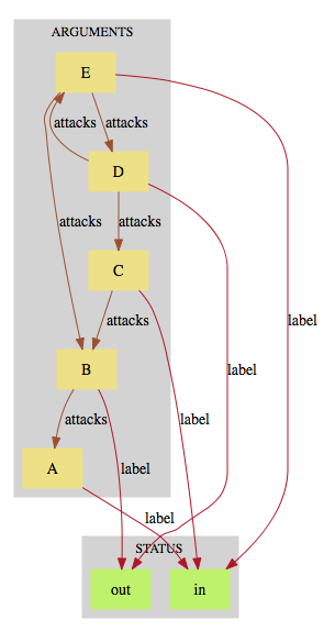
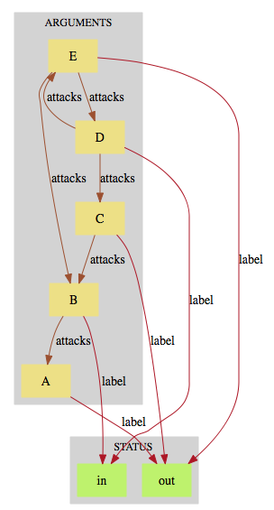
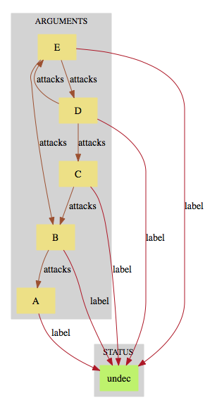
You can try and experiment with various attack graphs by editing the file. E.g., with

attacks = {B|->A, C|->B, D|->C, E |-> B, E|->D, D|->E} 

you now get three possible labelling, the last one assigns undec to all arguments.

A more elegant encoding

The following is a slightly more elegant encoding, where we represent the labelling as a partition of the arguments. This enables to use the relational image operator to express some constraints more compactly. This model is particularly well suited if you wish to use our Kodkod backend which translates the constraints to SAT. However, even the standard ProB solver can solve this instance in 10 ms (Kodkod requires 70 ms), so this would only be worthwhile for larger problem instances.

In case you are new to B, you probably need to know the following additional operators to understand the specification below (we als have a summary page about the B syntax):

• r~ is the inverse of a function or relation r
• r[S] is the relational image of a relation r for a set of domain values S

MACHINE ArgumentationAsSets
SETS
 ARGUMENTS={A,B,C,D,E}
CONSTANTS attacks, in,out,undec
PROPERTIES
  attacks : ARGUMENTS <-> ARGUMENTS  /* which argument attacks which other argument */
  &
  // we partition the arguments into three sets
  ARGUMENTS = in \/ out \/ undec &
  in /\ out = {} & in /\ undec = {} & out /\ undec = {} &
  
  // if an argument is in, any attacker must be out:
  attacks~[in] <: out &
  // if an argument is in, anything it attacks must be out: 
  attacks[in] <: out &
  //if an argument y is out, it must be attacked by a valid argument:
  !y.(y:out => #x.(x|->y:attacks & x:in)) & 
  // if an argument y is undecided, it must be attacked by an undecided argument:
  !y.(y:undec => #x.(x|->y:attacks & x:undec))

 &
  // here we model one particular argumentation graph
  // A = the sun will shine to day, B = we are in the UK, C = it is summer, D = there are only 10 days of sunshine per year, E = the BBC has forecast sun
  attacks = {B|->A, C|->B, D|->C, E |-> B, E|->D} 
END

Influencing the Graphical Rendering

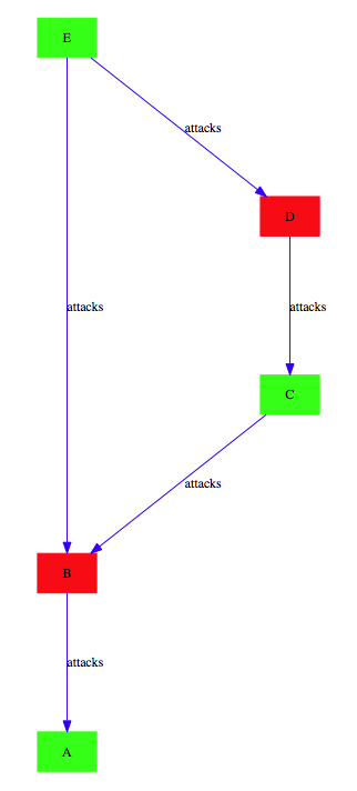
One can influence the graphical representation of the current state in various ways. The user can directly define nodes and edges of the graph to be rendered. One way to do this is by adding the following custom graph definition after the MACHINE section:

DEFINITIONS
 CUSTOM_GRAPH_NODES == (in * {"green"}) \/ (out * {"red"}) \/ (undec * {"orange"});
 CUSTOM_GRAPH_EDGES == attacks

These lines do not influence the meaning of the model; they are just used by ProB. Indeed, one can then use the "Current State as Custom Graph" command in the "States" submenu of the "Visualise" menu to obtain the following rendering of the very first example above:

An Event-B Version of the Model

Instead of using ProB Tcl/Tk you can also encode this model in Rodin, the Eclipse-based platform for Event-B.

Here we have split the model into two contexts. The first one encodes the general rules for labelling (we use Camille syntax):

context ArgumentsAsSets
sets ARGUMENTS
constants attacks in out undec
axioms
  @axm1 attacks ∈ ARGUMENTS ↔ ARGUMENTS // which argument attacks which other argument
  @axm2 partition(ARGUMENTS,in,out,undec)  // we partition the arguments into three sets
  @axm3 attacks∼[in] ⊆ out // if an argument is in, any attacker must be out
  @axm4 attacks[in] ⊆ out // if an argument is in, anything it attacks must be out
  @axm5 ∀y·(y∈out ⇒ ∃x·(x↦y∈attacks ∧ x∈in)) //if an argument y is out, it must be attacked by a valid argument
  @axm6 ∀y·(y∈undec ⇒ ∃x·(x↦y∈attacks ∧ x∈undec)) // if an argument y is undecided, it must be attacked by an undecided argument
end

A second context then extends the above one, and encodes our particular problem instance:

context Arguments_Example extends ArgumentsAsSets
constants A B C D E
axioms
  @part partition(ARGUMENTS,{A},{B},{C},{D},{E})
  @example attacks = {B↦A, C↦B, D↦C, E ↦ B, E↦D}
  /* A = the sun will shine to day, B = we are in the UK
     C = it is summer, D = there are only 10 days of sunshine per year, E = the BBC has forecast sun */
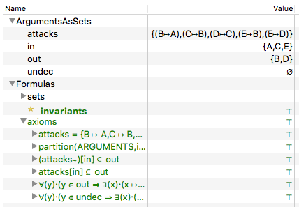
end

If you load this model with ProB for Rodin, you can see the solution in the State view: