Custom Graph: Difference between revisions
| Line 38: | Line 38: | ||
You can generate the custom graph for the current state in ProB Tcl/Tk by right-clicking in the "State Properties" pane and selecting "View State as Custom Graph" or by going to the State submenu of the Visualisation menu. You can also enter alternate custom graph records into the "Expression as Dot Graph" dialog in the Formulas submenu of the visualisation menu. | You can generate the custom graph for the current state in ProB Tcl/Tk by right-clicking in the "State Properties" pane and selecting "View State as Custom Graph" or by going to the State submenu of the Visualisation menu. You can also enter alternate custom graph records into the "Expression as Dot Graph" dialog in the Formulas submenu of the visualisation menu. | ||
In ProB2-UI you can view the custom graph via the "Graph Visualisation" dialog in the Visualisation menu ("Customized Current State as Graph" line). You can also add alternate custom graph record expressions into the "(Relational) Expression as Graph..." line. | |||
In [[probcli]] you can use the following command to create a custom graph (you can write to .dot, .svg or .pdf files): <tt>probcli IceCream_Generic.mch -init -dot custom_graph IceCream_Generic.pdf</tt>. | In [[probcli]] you can use the following command to create a custom graph (you can write to .dot, .svg or .pdf files): <tt>probcli IceCream_Generic.mch -init -dot custom_graph IceCream_Generic.pdf</tt>. | ||
Revision as of 09:24, 8 January 2024
You can visualise the state of an individual B, Z, TLA+ or Alloy model using custom graph definitions which are laid out using GraphViz.
Thereby it is possible to specify general graph attributes, the nodes and the edges of the graph.
There are various ways such a custom graph can be defined. The most powerful is providing a single DEFINITION called CUSTOM_GRAPH which defines global graph properties as well as defines nodes and edges.
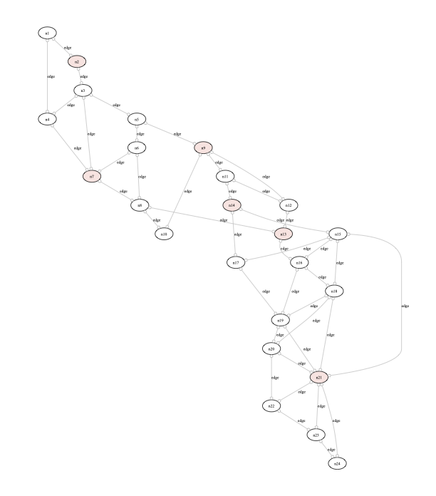
Suppose we have a B model with a binary relation edge and a set NODES as well as a total function ice from these nodes to BOOL. Here is an example custom graph definition:
 CUSTOM_GRAPH == rec(layout:"dot", rankdir:"TB",
                     nodes: {j•j:NODES |
                               rec(value:j, style:"filled",
                                fillcolor:IF ice(j)=TRUE THEN "mistyrose" ELSE "white" END
                                  )},
                    edges:rec(color:"gray", arrowhead:"odot",
                              arrowtail:"odot", dir:"both",
                              label:"edge",
                              edges: edge)
                    );
Here layout and rankdir are GraphViz attributes for the entire graph. Other values, e.g., for layout are: neato, circo, fdp, sfdp, twopi, patchwork, nop, nop2. Values for rankdir are: TB, BT, LR, RL. More graph attributes can be found here: [1].
The nodes field specifies the nodes of our graph. Here nodes evaluates to a set of records with the value field specifying the B identity of the node and the other fields style and fillcolor being GraphViz attributes. Supported attributes for nodes can be found here: [2]. Note that there can be other nodes fields, called nodes0, nodes1, ..., nodes9.
The edges field here is itself a record with GraphViz attributes. These are default attributes for the edges field, which here is a straightforward B relation (but it could again be a set of records with attributes). We could have used a similar record with default attributes in the nodes description above. Supported attributes for edges can be found here: [3]. Note that there can be other edges fields, called edges0, ..., edges9.
Generating Custom Graphs
You can generate the custom graph for the current state in ProB Tcl/Tk by right-clicking in the "State Properties" pane and selecting "View State as Custom Graph" or by going to the State submenu of the Visualisation menu. You can also enter alternate custom graph records into the "Expression as Dot Graph" dialog in the Formulas submenu of the visualisation menu.
In ProB2-UI you can view the custom graph via the "Graph Visualisation" dialog in the Visualisation menu ("Customized Current State as Graph" line). You can also add alternate custom graph record expressions into the "(Relational) Expression as Graph..." line.
In probcli you can use the following command to create a custom graph (you can write to .dot, .svg or .pdf files): probcli IceCream_Generic.mch -init -dot custom_graph IceCream_Generic.pdf.
The resulting visualisation (File:IceCream Generic.pdf) can be seen here:

In probcli you can also use the command --dotexpr expr_as_graph Formula File to visualise alternate custom graph records.
Full Example
The full model for experimentation is below. Some of the examples in the user manual also use this feature, for example the Bridges Puzzle (Hashiwokakero) (Jupyter notebook) or the Argumentation Theory example. These examples may use the older style definition, with two separate definitions CUSTOM_GRAPH_NODES and CUSTOM_GRAPH_EDGES, which is also supported by ProB.
MACHINE IceCream_Generic
//  a dominating set example:
// place ice cream vans so that every house (node) is at most one block away from a van
DEFINITIONS
 N == 24;
 CUSTOM_GRAPH == rec(layout:"dot", rankdir:"TB",
                     nodes: {j•j:NODES |
                               rec(value:j, style:"filled",
                                fillcolor:IF ice(j)=TRUE THEN "mistyrose" ELSE "white" END
                                  )},
                    edges:rec(color:"gray", arrowhead:"odot",
                              arrowtail:"odot", dir:"both",
                              label:"edge",
                              edges: edge)
                    );

      bi_edge == (edge \/ edge~);

  SET_PREF_SMT == TRUE;
  SET_PREF_TIME_OUT == 50000;
  SET_PREF_SOLVER_STRENGTH == 300;
  SET_PREF_SOLVER_FOR_PROPERTIES == "prob";
SETS
  NODES = {n1,n2,n3,n4,n5,n6,n7,n8,n9,n10,
           n11,n12,n13,n14,n15,n16,n17,n18,n19,n20,n21,n22,n23,n24}
CONSTANTS edge, ice, vans, neighbours
PROPERTIES
 edge: NODES <-> NODES &
 edge = { n1|->n2, n1|->n4,
          n2|->n3,
          n3|->n4, n3|->n5, n3|->n7,
          n4|->n7,
          n5|->n6, n5|->n9,
          n6|->n7, n6|->n8,
          n7|->n8,
          n8|->n10, n8|->n13,
          n9|->n10, n9|->n11, n9|->n12,
          n11|->n12, n11|->n14,
          n12|->n13,
          n13|->n16,
          n14|->n15, n14|->n17,
          n15|->n16, n15|->n17, n15|->n18, n15|->n21,
          n16|->n18, n16|->n19,
          n17|->n19,
          n18|->n19, n18|->n20, n18|->n21,
          n19|->n20, n19|->n21,
          n20|->n21, n20|->n22,
          n21|->n22, n21|->n23, n21|->n24,
          n22|->n23, n21|->n24,
          n23|->n24
          } &
 ice : NODES--> BOOL &
 neighbours = %x.(x:NODES|bi_edge[{x}]) &
 !x.(x:NODES =>
      (ice(x)=TRUE or
        #neighbour.(neighbour: neighbours(x) & ice(neighbour)=TRUE)
                 )
    )

 & vans = card(ice~[{TRUE}])
 & card({x|x:NODES & ice(x)=TRUE})<=6
  /* minimal solution requires 6 vans */

OPERATIONS
  v <-- NrVans = BEGIN v := vans END;
  xx <-- Get(yy) = PRE yy:NODES THEN xx:= ice(yy) END;
  v <-- Vans = BEGIN v:= ice~[{TRUE}] END
END