Argumentation Theory: Difference between revisions

Below we try to model some concepts of argumentation theory in B. The examples try to show that set theory can be used to model some aspects of argumentation theory quite naturally, and that ProB can solve and visualise some problems in argumentation theory. Alternative solutions are encoding arguments as normal logic programs and using answer set solvers for problem solving.

The following model was inspired by a talk given by Claudia Schulze.

The model below represents the labelling of the arguments as a total function from arguments to its status, which can either be in (the argument is accepted), out (the argument is rejected), or undec (the argument is undecided). The relation between the arguments is given in the binary attacks relation.

In case you are new to B, you probably need to know the following operators to understand the specification below (we als have a summary page about the B syntax):

• x : S specifies that x is an element of S
• a|->b represents the pair (a,b); note that a relation and function in B is a set of pairs.
• x|->y : R hence specifies that x is mapped to y in relation R
• !x.(P => Q) denotes universal quantification over variable x
• #x.(P & Q) denotes universal quantification over variable x
• A <--> B denotes the set of relations from A to B
• A --> B denotes the set of total functions from A to B

MACHINE ArgumentationTotFun
SETS
 ARGUMENTS={A,B,C,D,E};
 STATUS = {in,out,undec}
CONSTANTS attacks, label
PROPERTIES
  attacks : ARGUMENTS <-> ARGUMENTS  /* which argument attacks which other argument */
  &
  label: ARGUMENTS --> {in,out,undec} & /* the labeling function */
  !(x,y).(x|->y:attacks => (label(y)=in => label(x)=out)) &
  !(x).(x:ARGUMENTS => (label(x)=out => #y.(y|->x:attacks & label(y)=in))) &
  !(x,y).(x|->y:attacks => (label(y)=undec => label(x)/=in)) &
  !(x).(x:ARGUMENTS => (label(x)=undec => #y.(y|->x:attacks & label(y)=undec)))

 &
  // here we model one particular argumentation graph
  // A = the sun will shine to day, B = we are in the UK, C = it is summer, D = there are only 10 days of sunshine per year, E = the BBC has forecast sun
  attacks = {B|->A, C|->B, D|->C, E |-> B, E|->D} 
END

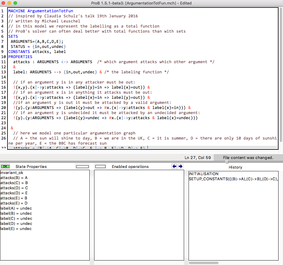
Here is a screenshot of ProB Tcl/Tk after loading the model.

You can see that there is only a single solution (solving time 10 ms), as only a single SETUP_CONSTANTS line is available in the "Enabled Operations" pane. Double-click on SETUP_CONSTANTS and then INITIALISATION will give you the following result, where you can see the solution in the "State Properties" pane:

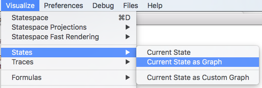
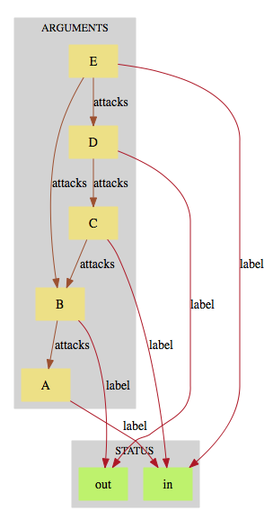
If you want to inspect the solution visually, you can select the "Current State as Graph" command in the "States" submenu of the "Visualize" menu:

This results in the following picture being displayed: